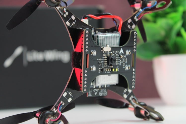
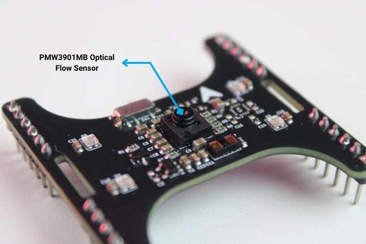
The LiteWing Flight Positioning Module uses the PMW3901MB optical flow sensor to measure horizontal motion relative to the ground. Instead of relying on GPS, this sensor tracks visual features on the surface beneath the drone and reports how those features move between frames. With the right processing, this information can be converted into velocity and approximate position in the X-Y plane. Check our advanced drone projects featuring autonomous flight, object tracking, and smart sensors for enhanced performance.
This guide explains the principle of operation and how the data exposed by LiteWing firmware can be used in your own scripts. The practical goal is to transform raw pixel deltas (deltaX, deltaY) into velocity and subsequently into 2D trajectory estimates.
Table of Contents
- Hardware Setup
- Software Setup
- How Optical Flow Works
- Optical Flow Velocity Calculation
- Position Estimation by Integration
- CRTP Communication for Optical Flow Data
- Velocity Calculation
- Code Walkthrough (test_optical_flow_sensor.py)
- └ GitHub Repository
- └ Connection Class and Data Structures
- └ Velocity Calculation
- └ Smoothing with an IIR Filter
- └ Log Callback and Position Integration
- └ Velocity and Trajectory Plotting
- Testing the Script Output
Hardware Setup
If you have not yet installed the LiteWing Drone Flight Positioning Module or updated the drone’s firmware to support the module, refer to the Flight Positioning Module User Guide. That document covers hardware installation and firmware flashing steps. Make sure your drone is running the Module-compatible firmware before continuing.
Software Setup
Before proceeding with any coding examples, it is important that your development environment is properly set up. This includes installing Python, configuring the required libraries, and ensuring that your PC can establish a CRTP link with the LiteWing. Since cflib has a few prerequisites that must be met, refer to the LiteWing Python SDK Programming Guide. That document provides detailed instructions for installing dependencies, setting up cflib, connecting to the LiteWing Wi-Fi interface, and validating communication with a simple test script. Completing that setup is necessary before attempting to interact with any sensor on the Flight Positioning Module.
Once the Python environment is ready and the connection to the drone is verified, we can move on to reading altitude data and comparing the fused and raw measurements in real time.
How Optical Flow Works
The PMW3901MB operates in a similar way to an optical mouse sensor, but with optics designed for far-field surfaces such as floors and ground textures. The sensor continually captures low-resolution images of the area below the drone. For each new frame, it compares the current image with the previous one and determines how far the pattern has shifted in the X and Y directions.
Internally, the sensor runs this process at roughly 200 frames per second. For each frame pair, it estimates how many pixels the image has moved horizontally (deltaX) and vertically (deltaY). If the image shifts by +10 pixels to the right between two frames, the reported deltaX is +10. If it shifts by -5 pixels downward, deltaY would be -5. These pixel deltas are accumulated and exposed through the SPI interface and, in the LiteWing firmware, mapped into log variables that can be streamed over CRTP.
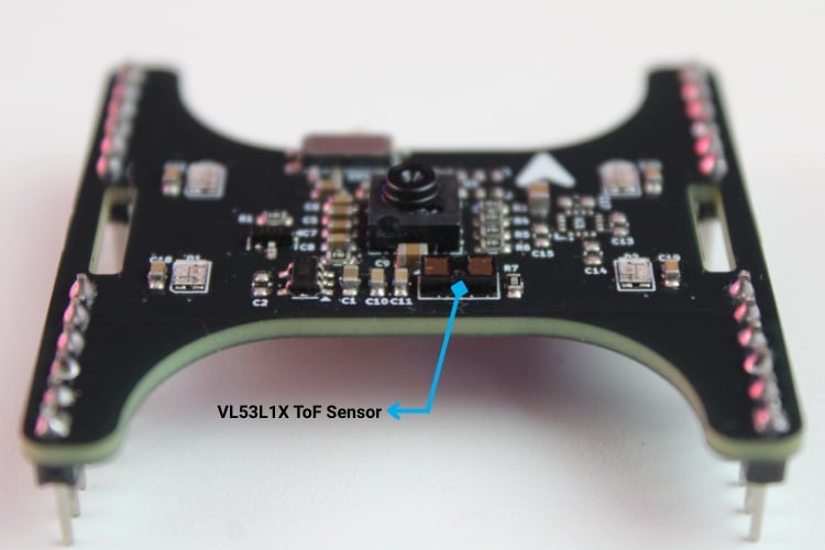
One important detail is that pixel motion alone does not directly give real-world velocity. A given pixel shift corresponds to different linear motion at different altitudes. A delta of 10 pixels in one frame when the drone is flying at 10 cm above the ground represents a much faster linear motion than the same 10 pixels at 1 m altitude. This is why the optical flow sensor is typically used together with a height measurement source, such as the VL53L1X Time-of-Flight sensor.
Optical Flow Velocity Calculation
The PMW3901MB optical flow sensor provides motion information in the form of pixel deltas. For each sampling interval, the sensor reports how many pixels the ground texture moved in the X and Y directions. These values alone do not indicate real-world speed, because the same pixel shift corresponds to different physical motion at different altitudes. To convert the sensor’s pixel motion into linear velocity, the LiteWing implementation combines three elements:
- Raw pixel deltas (Δx, Δy) from the optical flow sensor
- Altitude above the ground, obtained from the VL53L1X or state estimator
- A geometry constant derived from the sensor’s optics and frame rate
These are combined into a simple proportional relationship:
![]()
![]()
where:
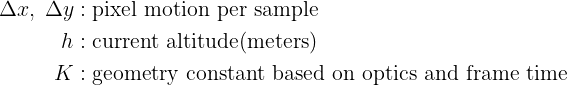
The PMW3901MB has an effective field-of-view of roughly 5.4°, spreads this across 30 pixels, and internally refreshes its frame at around 5 ms intervals. These parameters define how much angular motion each pixel represents and how often those angles are sampled. When combined, they form the proportional constant:
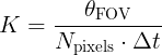
Where:
This constant converts pixel motion into an angular rate, which is then projected to a linear velocity using altitude.
Why Altitude Matters
Optical flow measures angular motion rather than absolute distance. For a given angular change, a small object that is close to the sensor will traverse a large number of pixels in the image, whereas the same object located farther away will traverse fewer pixels. Consequently, to maintain the same observed optical flow, linear velocity must scale with altitude.
![]()
This is why the LiteWing implementation always reads altitude together with deltaX/deltaY.
Smoothing and Noise Suppression
Pixel deltas from optical flow can vary by several percent even during steady motion. To produce a stable velocity estimate, we use a lightweight exponential smoothing filter:
![]()
where:
- α ≈ 0.7 in typical use
- Higher α = smoother but slightly slower response
- Very small velocities below a threshold are suppressed to avoid position drift
This approach removes jitter without introducing heavy lag, which is important for real-time navigation.
Position Estimation by Integration

This produces a 2D trajectory relative to the starting point. Over long durations, drift accumulates, as expected for any system based solely on dead-reckoning, but over short motion cycles, this method gives a useful representation of the drone’s path.
CRTP Communication for Optical Flow Data
To work with the optical flow sensor from your PC, the LiteWing firmware exposes motion-related data through CRTP log variables. For optical flow-based navigation, the main variables we use are the pixel shifts in X and Y, a surface quality metric, and the estimated altitude. These are streamed over the cflib logging interface in the same way as the height data from the previous guide.
Log Variables and Streaming
The following variables are read from the drone:
| motion.deltaX | Pixel shift in X direction (integer) |
| motion.deltaY | Pixel shift in Y direction (integer) |
| motion.squal | Feature confidence 0-255 (integer) |
| stateEstimate.z | Altitude (meters, needed for velocity conversion) |
motion.deltaX and motion.deltaY comes directly from the PMW3901MB optical flow sensor and represents how many pixels the ground pattern has moved between samples motion.squal is a confidence value that indicates how well the sensor is tracking features. stateEstimate.z is the fused altitude estimate, which is required to convert pixel shifts into real-world linear velocity.
Velocity Calculation
The optical flow sensor itself can only report motion in pixel units. To turn these into velocities in meters per second, we need altitude and a geometric scale factor that depends on the sensor’s optics.
In simplified form, the conversion is:
velocity (m/s) = deltaX (pixels) × altitude (m) × geometry_constant
In the script, this constant is defined as:
 velocity_constant = (5.4 * DEG_TO_RAD) / (30.0 * DT)    # 5.4° = sensor field of view 30   = pixel resolution DT   = sample time (5 ms typical)
   return delta_value * altitude_m * velocity_constant
This packs the sensor’s angular field of view, resolution, and sample interval into a single scalar used for velocity computation. In practice, this constant is often tuned experimentally to match observed motion.
Surface Quality Metric
The motion.squal variable (0-255) indicates how reliable the current optical flow measurement is. Higher values correspond to surfaces with clear features and good lighting; low values indicate poor tracking conditions.
| Range | Interpretation |
| 0-50 | Poor: flat, glossy, or very dark surfaces |
| 50-150 | Fair: usable, but expect some noise and dropouts |
| 150-255 | Excellent: rich texture and good lighting |
When surface quality is consistently low, velocity and position estimates based on optical flow should not be trusted.
Code Walkthrough (test_optical_flow_sensor.py)
The test_optical_flow_sensor.py script demonstrates how to stream optical flow data from the LiteWing, convert pixel deltas to velocities, and integrate them into a 2D trajectory. It also plots both velocity and path in a simple GUI.
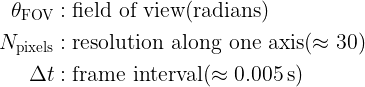
GitHub Repository and Source Files
You can get the script on our LiteWing GitHub repository under LiteWing/Python-Scripts/Flight_Positioning_Module/


Imports and Constants
The script starts by importing the required modules and defining a few constants for geometry, filtering, and orientation:
import math
import threading
import time
from collections import deque
import tkinter as tk
import matplotlib
matplotlib.use("TkAgg")
from matplotlib.backends.backend_tkagg import FigureCanvasTkAgg
from matplotlib.figure import Figure
import cflib.crtp
from cflib.crazyflie import Crazyflie
from cflib.crazyflie.log import LogConfig
from cflib.crazyflie.syncCrazyflie import SyncCrazyflie
DT = LOG_PERIOD_MS / 1000.0 # DT is the logging interval converted to seconds; used when integrating velocities to compute position displacement between samples.
DEG_TO_RAD = math.pi / 180.0 # conversion factor from degrees to radians
ALPHA = 0.7 # IIR smoothing factor for velocity values (0 < ALPHA < 1)
VELOCITY_THRESHOLD = 0.005  # m/s - velocities below this are clamped to zero
INVERT_X_AXIS_DEFAULT = True # sensor is mounted inverted on the LiteWing shield
HISTORY_LENGTH = 400 # number of samples to keep in history for plotting
The main constants are summarised below:
| Constant | Purpose |
| ALPHA | Weight for IIR smoothing (closer to 1 = smoother) |
| VELOCITY_THRESHOLD | Eliminates tiny residual velocities as noise |
| INVERT_X_AXIS_DEFAULT | Corrects the axis for the way the sensor is mounted |
Connection Class and Data Structures
The main logic is encapsulated in an OpticalFlowTest class. This object owns the Crazyflie instance, connection callbacks, and all motion-related states.
class OpticalFlowApp:
   def __init__(self, root: tk.Tk):
       self.root = root
       self.root.title("LiteWing Optical Flow Test")
       self.root.geometry("1100x760")
       # GUI state variables
       self.status_var = tk.StringVar(value="Status: Idle")
       self.delta_var = tk.StringVar(value="ΔX: 0, ΔY: 0")
       self.velocity_var = tk.StringVar(value="Velocity XY: 0.000, 0.000 m/s")
       self.height_var = tk.StringVar(value="Height: 0.000 m")
       self.squal_var = tk.StringVar(value="Surface Quality: 0")
       # Sensor mount is inverted in the LiteWing hardware; keep a fixed flag
       # to map the raw delta to the GUI reported value.
       self.invert_x = bool(INVERT_X_AXIS_DEFAULT)
       self._build_controls()
       self._build_plot()
       # Threading primitives to start/stop the logging thread and protect
       # access to the shared history variables used by GUI and the logger
       self.stop_event = threading.Event()
       self.connection_thread: threading.Thread | None = None
       self.data_lock = threading.Lock()
       # Circular buffers preserving a fixed amount of history for plotting
       self.time_history = deque(maxlen=HISTORY_LENGTH)
       self.vx_history = deque(maxlen=HISTORY_LENGTH)
       self.vy_history = deque(maxlen=HISTORY_LENGTH)
       # Integrated XY trajectory in meters computed by integrating velocities
       self.pos_x_history = deque(maxlen=HISTORY_LENGTH)
       self.pos_y_history = deque(maxlen=HISTORY_LENGTH)
       # Initialize smoothing history for each axis
       self.smoothed_vx = [0.0]
       self.smoothed_vy = [0.0]
       # Position integration state (meters)
       self.position_x = 0.0
       self.position_y = 0.0
The script uses fixed-length deques to store a rolling history of velocities, positions, and timestamps. This keeps memory usage bounded, while still providing enough history for plotting.
Log Configuration and Streaming
When the connection is established, the script sets up a log configuration for the motion variables and altitude. This is done in the _connection_worker callback.
 def _connection_worker(self) -> None:
       # This worker runs in a separate thread and does the radio I/O via the
       # cfclient library. It registers log variables, starts the log stream,
       # and then waits until the stop_event is triggered to clean up.
       self._set_status("Status: Connecting...")
       try:
           # Initialize the Crazyradio drivers (no debug radio by default)
           cflib.crtp.init_drivers(enable_debug_driver=False)
           with SyncCrazyflie(DRONE_URI, cf=Crazyflie(rw_cache="./cache")) as scf:
               cf = scf.cf
               self._set_status("Status: Connected")
               # Create a log config that retrieves sensor deltas and the
               # estimated height repeatedly at LOG_PERIOD_MS intervals.
               log_config = LogConfig(name="OpticalFlow", period_in_ms=LOG_PERIOD_MS)
               variables = [
                   ("motion.deltaX", "int16_t"),
                   ("motion.deltaY", "int16_t"),
                   ("motion.squal", "uint8_t"),
                   ("stateEstimate.z", "float"),
               ]
               # Query the CF TOC (Table of Contents) to ensure variables are
               # present in the running firmware, and add them to the log.
               if not self._add_variables_if_available(cf, log_config, variables):
                   self._set_status("Status: Optical flow variables unavailable")
                   return
               log_config.data_received_cb.add_callback(self._log_callback)
               cf.log.add_config(log_config)
               log_config.start()
               print("[Flow] Logging started")
A logging period of 50 ms (20 Hz) is used as a compromise between responsiveness and bandwidth. The PMW3901MB itself can update much faster, but streaming every sensor frame is unnecessary for visualization and basic position estimation.
Velocity Calculation
The core of the conversion from pixels to meters per second is handled in a small helper function:
def calculate_velocity(delta_value: int, altitude_m: float) -> float:
   """
   Convert a raw optical-flow delta reading into a velocity (m/s).
   The flow sensor gives pixel deltas per frame; to convert to meters per second
   we take into account the altitude above ground and the (approximate)
   optical geometry. The conversion is linear with altitude: at higher altitude,
   the same angular delta corresponds to a larger ground displacement.
   Args:
       delta_value: Raw integer optical-flow delta reported by sensor (counts).
       altitude_m: Estimated altitude in meters from the state estimator.
   Returns:
       Velocity in meters per second along the given axis.
   """
   # If altitude is not positive we can't compute velocity reliably
   if altitude_m <= 0:
       return 0.0
   # velocity_constant encodes conversion factors (sensor FoV, resolution,
   # and logging period) into a per-sample scaling factor.
   velocity_constant = (5.4 * DEG_TO_RAD) / (30.0 * DT)    # 5.4° = sensor field of view 30   = pixel resolution DT   = sample time (5 ms typical)
   return delta_value * altitude_m * velocity_constant
This function assumes a positive, non-zero altitude. For safety, altitude values at or below zero are treated as invalid, and the function returns zero velocity in that case.
Smoothing with an IIR Filter
To reduce noise without introducing heavy lag, an IIR low-pass filter is applied to the raw velocities:
def smooth_velocity(new_value: float, history: list[float]) -> float:
   """
   Simple IIR smoothing for velocity values.
   The function takes a new sample and a history list used to compute a
   first-order IIR (exponential) smoothing using alpha. The history is
   stored to allow the GUI to also display recent values. To avoid drift or
   reporting near-zero noise as movement, values below VELOCITY_THRESHOLD are
   clamped to zero.
   """
   history.append(new_value)
   if len(history) < 2:
       # Not enough history to smooth yet, return the raw value
       return new_value
   smoothed = history[-1] * ALPHA + history[-2] * (1 - ALPHA)
   # Reject very small velocities to avoid reacting to noise
   if abs(smoothed) < VELOCITY_THRESHOLD:
       return 0.0
   return smoothed
This filter gives a simple way to balance responsiveness and stability. The final clamping step is useful to avoid slow drift in position estimates when the drone is stationary.
Log Callback and Position Integration
The main data path runs in the _log_callback, which is invoked whenever a new log packet arrives:
  def _log_callback(self, timestamp: int, data: dict, _: LogConfig) -> None:
       delta_x = data.get("motion.deltaX", 0)
       delta_y = data.get("motion.deltaY", 0)
       squal = data.get("motion.squal", 0)
       altitude = data.get("stateEstimate.z", 0.0)
       # Sensor is mounted inverted; map delta_x accordingly (maps raw -> GUI)
       delta_x_mapped = -delta_x if self.invert_x else delta_x
       raw_vx = calculate_velocity(delta_x_mapped, altitude)
       raw_vy = calculate_velocity(delta_y, altitude)
       vx = smooth_velocity(raw_vx, self.smoothed_vx)
       vy = smooth_velocity(raw_vy, self.smoothed_vy)
       # Timestamp the sample to compute a true delta-time between events
       now = time.time()
       # Compute time since last sample; clamp to a sane max to avoid
       # integration jumps if sampling pauses.
       if self.last_sample_time is None:
           dt = DT
       else:
           dt = max(0.0, min(now - self.last_sample_time, 0.5))
       self.last_sample_time = now
       # Integrate velocity -> position using the measured time delta
       self.position_x += vx * dt
       self.position_y += vy * dt
       with self.data_lock:
           # Append new sample to each history buffer used for plotting
           self.time_history.append(now)
           self.vx_history.append(vx)
           self.vy_history.append(vy)
           self.pos_x_history.append(self.position_x)
           self.pos_y_history.append(self.position_y)
           # Store mapped delta_x since the GUI will show the mapped axis
           self.latest_values = (delta_x_mapped, delta_y, vx, vy, altitude, squal)
       if time.time() - self.last_console_print >= 1.0:
           self.last_console_print = time.time()
           # Print raw delta and computed velocities to the console every
           # second for fast debugging without relying on the GUI.
           print(
               f"[Flow] ΔX={delta_x} ΔY={delta_y} | VX={vx:.3f} m/s VY={vy:.3f} m/s | "
               f"Height={altitude:.3f} m | Squal={squal}"
           )
This function reads raw pixel deltas along with surface quality and altitude data, applies an orientation correction when the sensor is mounted in a flipped configuration, and converts the resulting pixel deltas into velocities expressed in meters per second. The computed velocities are then smoothed using an IIR filter and integrated over time to update the position_x and position_y state variables. Finally, the function stores the relevant values for subsequent plotting and outputs a summarized status at a reduced rate to support console-based debugging.
Velocity and Trajectory Plotting
The visualization part of the script uses Matplotlib embedded in a Tk window. The update_plot function updates both the velocity plot and the XY trajectory:
 def _build_plot(self) -> None:
       self.figure = Figure(figsize=(11, 6.5), dpi=100)
       self.ax_vel = self.figure.add_subplot(2, 1, 1)
       # First subplot shows the recent X/Y velocities (m/s)
       self.ax_vel.set_title("Velocities")
       self.ax_vel.set_ylabel("Velocity (m/s)")
       self.ax_vel.grid(True, alpha=0.3)
       (self.vx_line,) = self.ax_vel.plot([], [], label="VX", color="tab:red")
       (self.vy_line,) = self.ax_vel.plot([], [], label="VY", color="tab:green")
       self.ax_vel.legend(loc="upper right")
       self.ax_pos = self.figure.add_subplot(2, 1, 2)
       # Second subplot shows the integrated XY trajectory in meters
       self.ax_pos.set_title("Integrated Trajectory")
       self.ax_pos.set_xlabel("X (m)")
       self.ax_pos.set_ylabel("Y (m)")
       self.ax_pos.set_aspect("equal")
       self.ax_pos.grid(True, alpha=0.3)
       (self.trajectory_line,) = self.ax_pos.plot([], [], color="tab:blue", linewidth=2)
       (self.current_point,) = self.ax_pos.plot([], [], marker="o", color="tab:orange")
       canvas = FigureCanvasTkAgg(self.figure, master=self.root)
       canvas.draw()
       canvas.get_tk_widget().pack(fill=tk.BOTH, expand=True, padx=10, pady=10)
       self.canvas = canvasdef _refresh_gui(self) -> None:
       with self.data_lock:
           if getattr(self, "latest_values", None):
               delta_x, delta_y, vx, vy, altitude, squal = self.latest_values
               self.delta_var.set(f"ΔX: {delta_x}, ΔY: {delta_y}")
               self.velocity_var.set(f"Velocity XY: {vx:.3f}, {vy:.3f} m/s")
               self.height_var.set(f"Height: {altitude:.3f} m")
               self.squal_var.set(f"Surface Quality: {squal}")
               # Build relative time axis for plotting
               times = list(self.time_history)
               if times:
                   t0 = times[0]
                   rel_times = [t - t0 for t in times]
                   vx_vals = list(self.vx_history)
                   vy_vals = list(self.vy_history)
                   pos_x = list(self.pos_x_history)
                   pos_y = list(self.pos_y_history)
                   # Update lines for velocities
                   self.vx_line.set_data(rel_times, vx_vals)
                   self.vy_line.set_data(rel_times, vy_vals)
                   # Keep the right-most 20 seconds visible in the velocity
                   # subplot for context while streaming.
                   last_time = rel_times[-1] if rel_times[-1] > 1 else 1
                   self.ax_vel.set_xlim(max(0, last_time - 20), last_time + 1)
                   # Combine velocities to compute symmetrical Y limits around
                   # the current min/max so the plots remain stable.
                   combined_vel = vx_vals + vy_vals
                   vmin = min(combined_vel) if combined_vel else -0.1
                   vmax = max(combined_vel) if combined_vel else 0.1
                   margin = max(0.05, (vmax - vmin) * 0.2)
                   self.ax_vel.set_ylim(vmin - margin, vmax + margin)
                   # Update trajectory plot with integrated positions (meters).
                   self.trajectory_line.set_data(pos_x, pos_y)
                   if pos_x and pos_y:
                       self.current_point.set_data([pos_x[-1]], [pos_y[-1]])
                       # Auto-zoom and center the trajectory plot while
                       # maintaining aspect ratio for accurate XY scaling.
                       xmin, xmax = min(pos_x), max(pos_x)
                       ymin, ymax = min(pos_y), max(pos_y)
                       span_x = max(0.1, xmax - xmin)
                       span_y = max(0.1, ymax - ymin)
                       center_x = (xmin + xmax) / 2
                       center_y = (ymin + ymax) / 2
                       pad_x = span_x * 0.4
                       pad_y = span_y * 0.4
                       self.ax_pos.set_xlim(center_x - pad_x, center_x + pad_x)
                       self.ax_pos.set_ylim(center_y - pad_y, center_y + pad_y)
                   self.canvas.draw_idle()
The upper plot shows the smoothed velocities in X and Y over time. The lower plot shows the integrated XY path, marking the origin and current position, and maintaining a square aspect ratio so that distances are represented consistently along both axes.
Testing the Script Output
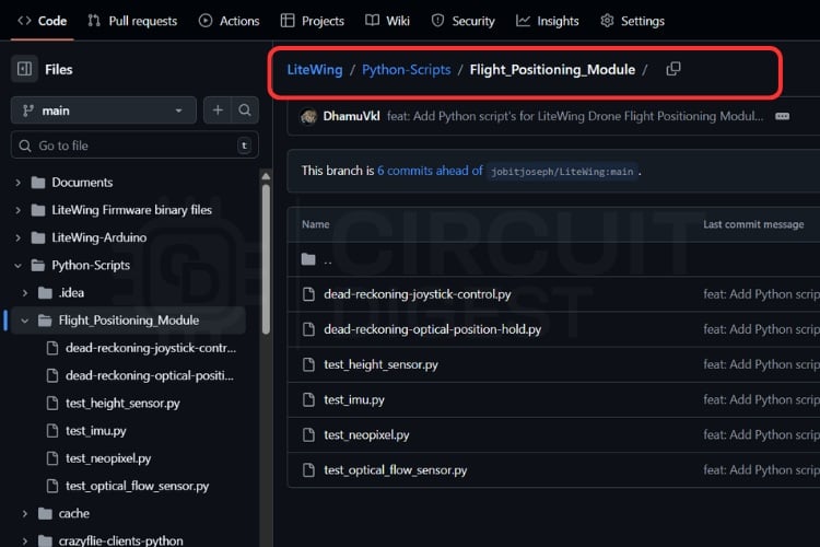
After launching the script and connecting to the LiteWing, it will start streaming optical flow and altitude data, and the GUI window begins updating in real time.
With the drone placed on the ground and kept stationary, the values shown in the UI should remain close to zero. The pixel deltas (ΔX, ΔY) fluctuate slightly due to sensor noise, but the computed velocities remain near zero after smoothing. The trajectory plot stays centered around the origin, confirming that the system is not integrating noise into position drift.
To verify motion tracking, gently move the drone by hand over the surface and perform a slow, controlled hover close to the ground. As the drone is translated forward, backwards, left, or right, the pixel delta values change immediately. Corresponding velocity values appear in the UI, and the trajectory plot begins to extend in the direction of motion. When the movement stops, velocities decay back to zero, and the plotted position remains at its last value.
Document Index
Complete Project Code
"""Standalone optical flow sensor test for the LiteWing flight Positioning Module.
Streams raw optical flow deltas, computed velocities, and the integrated XY
trajectory to both the console and a matplotlib-enabled Tk GUI.
"""
import math
import threading
import time
from collections import deque
import tkinter as tk
import matplotlib
matplotlib.use("TkAgg")
from matplotlib.backends.backend_tkagg import FigureCanvasTkAgg
from matplotlib.figure import Figure
import cflib.crtp
from cflib.crazyflie import Crazyflie
from cflib.crazyflie.log import LogConfig
from cflib.crazyflie.syncCrazyflie import SyncCrazyflie
DRONE_URI = "udp://192.168.43.42"
LOG_PERIOD_MS = 50 # 20 Hz logging interval
DT = LOG_PERIOD_MS / 1000.0 # DT is the logging interval converted to seconds; used when integrating velocities to compute position displacement between samples.
DEG_TO_RAD = math.pi / 180.0 # conversion factor from degrees to radians
ALPHA = 0.7 # IIR smoothing factor for velocity values (0 < ALPHA < 1)
VELOCITY_THRESHOLD = 0.005  # m/s - velocities below this are clamped to zero
INVERT_X_AXIS_DEFAULT = True # sensor is mounted inverted on the LiteWing shield
HISTORY_LENGTH = 400 # number of samples to keep in history for plotting
def calculate_velocity(delta_value: int, altitude_m: float) -> float:
   """
   Convert a raw optical-flow delta reading into a velocity (m/s).
   The flow sensor gives pixel deltas per frame; to convert to meters per second
   we take into account the altitude above ground and the (approximate)
   optical geometry. The conversion is linear with altitude: at higher altitude,
   the same angular delta corresponds to a larger ground displacement.
   Args:
       delta_value: Raw integer optical-flow delta reported by sensor (counts).
       altitude_m: Estimated altitude in meters from the state estimator.
   Returns:
       Velocity in meters per second along the given axis.
   """
   # If altitude is not positive we can't compute velocity reliably
   if altitude_m <= 0:
       return 0.0
   # velocity_constant encodes conversion factors (sensor FoV, resolution,
   # and logging period) into a per-sample scaling factor.
   velocity_constant = (5.4 * DEG_TO_RAD) / (30.0 * DT)    # 5.4° = sensor field of view 30   = pixel resolution DT   = sample time (5 ms typical)
   return delta_value * altitude_m * velocity_constant
def smooth_velocity(new_value: float, history: list[float]) -> float:
   """
   Simple IIR smoothing for velocity values.
   The function takes a new sample and a history list used to compute a
   first-order IIR (exponential) smoothing using alpha. The history is
   stored to allow the GUI to also display recent values. To avoid drift or
   reporting near-zero noise as movement, values below VELOCITY_THRESHOLD are
   clamped to zero.
   """
   history.append(new_value)
   if len(history) < 2:
       # Not enough history to smooth yet, return the raw value
       return new_value
   smoothed = history[-1] * ALPHA + history[-2] * (1 - ALPHA)
   # Reject very small velocities to avoid reacting to noise
   if abs(smoothed) < VELOCITY_THRESHOLD:
       return 0.0
   return smoothed
class OpticalFlowApp:
   def __init__(self, root: tk.Tk):
       self.root = root
       self.root.title("LiteWing Optical Flow Test")
       self.root.geometry("1100x760")
       # GUI state variables
       self.status_var = tk.StringVar(value="Status: Idle")
       self.delta_var = tk.StringVar(value="ΔX: 0, ΔY: 0")
       self.velocity_var = tk.StringVar(value="Velocity XY: 0.000, 0.000 m/s")
       self.height_var = tk.StringVar(value="Height: 0.000 m")
       self.squal_var = tk.StringVar(value="Surface Quality: 0")
       # Sensor mount is inverted in the LiteWing hardware; keep a fixed flag
       # to map the raw delta to the GUI reported value.
       self.invert_x = bool(INVERT_X_AXIS_DEFAULT)
       self._build_controls()
       self._build_plot()
       # Threading primitives to start/stop the logging thread and protect
       # access to the shared history variables used by GUI and the logger
       self.stop_event = threading.Event()
       self.connection_thread: threading.Thread | None = None
       self.data_lock = threading.Lock()
       # Circular buffers preserving a fixed amount of history for plotting
       self.time_history = deque(maxlen=HISTORY_LENGTH)
       self.vx_history = deque(maxlen=HISTORY_LENGTH)
       self.vy_history = deque(maxlen=HISTORY_LENGTH)
       # Integrated XY trajectory in meters computed by integrating velocities
       self.pos_x_history = deque(maxlen=HISTORY_LENGTH)
       self.pos_y_history = deque(maxlen=HISTORY_LENGTH)
       # Initialize smoothing history for each axis
       self.smoothed_vx = [0.0]
       self.smoothed_vy = [0.0]
       # Position integration state (meters)
       self.position_x = 0.0
       self.position_y = 0.0
       self.last_sample_time: float | None = None
       self.last_console_print = 0.0
       # Schedule periodic GUI updates
       self.root.after(100, self._refresh_gui)
       self.root.protocol("WM_DELETE_WINDOW", self._on_close)
   def _build_controls(self) -> None:
       top_frame = tk.Frame(self.root)
       top_frame.pack(fill=tk.X, padx=10, pady=6)
       # Start/Stop buttons to open/close the radio connection and begin
       # logging from the flight Positioning flow sensor.
       tk.Button(top_frame, text="Start", command=self.start, bg="#28a745", fg="white", width=12).pack(side=tk.LEFT, padx=5)
       tk.Button(top_frame, text="Stop", command=self.stop, bg="#dc3545", fg="white", width=12).pack(side=tk.LEFT, padx=5)
       tk.Label(top_frame, textvariable=self.status_var, font=("Arial", 11, "bold"), fg="blue").pack(side=tk.LEFT, padx=20)
       value_frame = tk.Frame(self.root)
       value_frame.pack(fill=tk.X, padx=10, pady=6)
       tk.Label(value_frame, textvariable=self.delta_var, font=("Arial", 12)).pack(side=tk.LEFT, padx=10)
       tk.Label(value_frame, textvariable=self.velocity_var, font=("Arial", 12)).pack(side=tk.LEFT, padx=10)
       tk.Label(value_frame, textvariable=self.height_var, font=("Arial", 12)).pack(side=tk.LEFT, padx=10)
       tk.Label(value_frame, textvariable=self.squal_var, font=("Arial", 12)).pack(side=tk.LEFT, padx=10)
   def _build_plot(self) -> None:
       self.figure = Figure(figsize=(11, 6.5), dpi=100)
       self.ax_vel = self.figure.add_subplot(2, 1, 1)
       # First subplot shows the recent X/Y velocities (m/s)
       self.ax_vel.set_title("Velocities")
       self.ax_vel.set_ylabel("Velocity (m/s)")
       self.ax_vel.grid(True, alpha=0.3)
       (self.vx_line,) = self.ax_vel.plot([], [], label="VX", color="tab:red")
       (self.vy_line,) = self.ax_vel.plot([], [], label="VY", color="tab:green")
       self.ax_vel.legend(loc="upper right")
       self.ax_pos = self.figure.add_subplot(2, 1, 2)
       # Second subplot shows the integrated XY trajectory in meters
       self.ax_pos.set_title("Integrated Trajectory")
       self.ax_pos.set_xlabel("X (m)")
       self.ax_pos.set_ylabel("Y (m)")
       self.ax_pos.set_aspect("equal")
       self.ax_pos.grid(True, alpha=0.3)
       (self.trajectory_line,) = self.ax_pos.plot([], [], color="tab:blue", linewidth=2)
       (self.current_point,) = self.ax_pos.plot([], [], marker="o", color="tab:orange")
       canvas = FigureCanvasTkAgg(self.figure, master=self.root)
       canvas.draw()
       canvas.get_tk_widget().pack(fill=tk.BOTH, expand=True, padx=10, pady=10)
       self.canvas = canvas
   def start(self) -> None:
       # If the background connection thread is already running, do nothing
       if self.connection_thread and self.connection_thread.is_alive():
           return
       self.stop_event.clear()
       # Spawn a background thread which manages the Crazyflie connection
       # and receives logged optical flow data without blocking the GUI.
       self.connection_thread = threading.Thread(target=self._connection_worker, daemon=True)
       self.connection_thread.start()
   def stop(self) -> None:
       self.stop_event.set()
   def _connection_worker(self) -> None:
       # This worker runs in a separate thread and does the radio I/O via the
       # cfclient library. It registers log variables, starts the log stream,
       # and then waits until the stop_event is triggered to clean up.
       self._set_status("Status: Connecting...")
       try:
           # Initialize the Crazyradio drivers (no debug radio by default)
           cflib.crtp.init_drivers(enable_debug_driver=False)
           with SyncCrazyflie(DRONE_URI, cf=Crazyflie(rw_cache="./cache")) as scf:
               cf = scf.cf
               self._set_status("Status: Connected")
               # Create a log config that retrieves sensor deltas and the
               # estimated height repeatedly at LOG_PERIOD_MS intervals.
               log_config = LogConfig(name="OpticalFlow", period_in_ms=LOG_PERIOD_MS)
               variables = [
                   ("motion.deltaX", "int16_t"),
                   ("motion.deltaY", "int16_t"),
                   ("motion.squal", "uint8_t"),
                   ("stateEstimate.z", "float"),
               ]
               # Query the CF TOC (Table of Contents) to ensure variables are
               # present in the running firmware, and add them to the log.
               if not self._add_variables_if_available(cf, log_config, variables):
                   self._set_status("Status: Optical flow variables unavailable")
                   return
               log_config.data_received_cb.add_callback(self._log_callback)
               cf.log.add_config(log_config)
               log_config.start()
               print("[Flow] Logging started")
               # Wait/multiplex until the GUI signals stop via stop_event.
               while not self.stop_event.is_set():
                   time.sleep(0.1)
               log_config.stop()
               print("[Flow] Logging stopped")
       except Exception as exc:  # noqa: BLE001
           print(f"[Flow] Connection error: {exc}")
           self._set_status("Status: Error - check console")
       finally:
           self._set_status("Status: Idle")
   def _add_variables_if_available(self, cf: Crazyflie, log_config: LogConfig, candidates: list[tuple[str, str]]) -> bool:
       # Access the Crazyflie Log TOC which describes available log variables
       toc = cf.log.toc.toc
       added = 0
       for full_name, var_type in candidates:
           group, name = full_name.split(".", maxsplit=1)
           if group in toc and name in toc[group]:
               log_config.add_variable(full_name, var_type)
               print(f"[Flow] Logging {full_name}")
               added += 1
           else:
               print(f"[Flow] Missing {full_name}")
       return added > 0
   def _log_callback(self, timestamp: int, data: dict, _: LogConfig) -> None:
       delta_x = data.get("motion.deltaX", 0)
       delta_y = data.get("motion.deltaY", 0)
       squal = data.get("motion.squal", 0)
       altitude = data.get("stateEstimate.z", 0.0)
       # Sensor is mounted inverted; map delta_x accordingly (maps raw -> GUI)
       delta_x_mapped = -delta_x if self.invert_x else delta_x
       raw_vx = calculate_velocity(delta_x_mapped, altitude)
       raw_vy = calculate_velocity(delta_y, altitude)
       vx = smooth_velocity(raw_vx, self.smoothed_vx)
       vy = smooth_velocity(raw_vy, self.smoothed_vy)
       # Timestamp the sample to compute a true delta-time between events
       now = time.time()
       # Compute time since last sample; clamp to a sane max to avoid
       # integration jumps if sampling pauses.
       if self.last_sample_time is None:
           dt = DT
       else:
           dt = max(0.0, min(now - self.last_sample_time, 0.5))
       self.last_sample_time = now
       # Integrate velocity -> position using the measured time delta
       self.position_x += vx * dt
       self.position_y += vy * dt
       with self.data_lock:
           # Append new sample to each history buffer used for plotting
           self.time_history.append(now)
           self.vx_history.append(vx)
           self.vy_history.append(vy)
           self.pos_x_history.append(self.position_x)
           self.pos_y_history.append(self.position_y)
           # Store mapped delta_x since the GUI will show the mapped axis
           self.latest_values = (delta_x_mapped, delta_y, vx, vy, altitude, squal)
       if time.time() - self.last_console_print >= 1.0:
           self.last_console_print = time.time()
           # Print raw delta and computed velocities to the console every
           # second for fast debugging without relying on the GUI.
           print(
               f"[Flow] ΔX={delta_x} ΔY={delta_y} | VX={vx:.3f} m/s VY={vy:.3f} m/s | "
               f"Height={altitude:.3f} m | Squal={squal}"
           )
   def _refresh_gui(self) -> None:
       with self.data_lock:
           if getattr(self, "latest_values", None):
               delta_x, delta_y, vx, vy, altitude, squal = self.latest_values
               self.delta_var.set(f"ΔX: {delta_x}, ΔY: {delta_y}")
               self.velocity_var.set(f"Velocity XY: {vx:.3f}, {vy:.3f} m/s")
               self.height_var.set(f"Height: {altitude:.3f} m")
               self.squal_var.set(f"Surface Quality: {squal}")
               # Build relative time axis for plotting
               times = list(self.time_history)
               if times:
                   t0 = times[0]
                   rel_times = [t - t0 for t in times]
                   vx_vals = list(self.vx_history)
                   vy_vals = list(self.vy_history)
                   pos_x = list(self.pos_x_history)
                   pos_y = list(self.pos_y_history)
                   # Update lines for velocities
                   self.vx_line.set_data(rel_times, vx_vals)
                   self.vy_line.set_data(rel_times, vy_vals)
                   # Keep the right-most 20 seconds visible in the velocity
                   # subplot for context while streaming.
                   last_time = rel_times[-1] if rel_times[-1] > 1 else 1
                   self.ax_vel.set_xlim(max(0, last_time - 20), last_time + 1)
                   # Combine velocities to compute symmetrical Y limits around
                   # the current min/max so the plots remain stable.
                   combined_vel = vx_vals + vy_vals
                   vmin = min(combined_vel) if combined_vel else -0.1
                   vmax = max(combined_vel) if combined_vel else 0.1
                   margin = max(0.05, (vmax - vmin) * 0.2)
                   self.ax_vel.set_ylim(vmin - margin, vmax + margin)
                   # Update trajectory plot with integrated positions (meters).
                   self.trajectory_line.set_data(pos_x, pos_y)
                   if pos_x and pos_y:
                       self.current_point.set_data([pos_x[-1]], [pos_y[-1]])
                       # Auto-zoom and center the trajectory plot while
                       # maintaining aspect ratio for accurate XY scaling.
                       xmin, xmax = min(pos_x), max(pos_x)
                       ymin, ymax = min(pos_y), max(pos_y)
                       span_x = max(0.1, xmax - xmin)
                       span_y = max(0.1, ymax - ymin)
                       center_x = (xmin + xmax) / 2
                       center_y = (ymin + ymax) / 2
                       pad_x = span_x * 0.4
                       pad_y = span_y * 0.4
                       self.ax_pos.set_xlim(center_x - pad_x, center_x + pad_x)
                       self.ax_pos.set_ylim(center_y - pad_y, center_y + pad_y)
                   self.canvas.draw_idle()
       self.root.after(100, self._refresh_gui)
   def _set_status(self, text: str) -> None:
       self.status_var.set(text)
   def _on_close(self) -> None:
       self.stop()
       self.root.after(200, self.root.destroy)
def main() -> None:
   root = tk.Tk()
   app = OpticalFlowApp(root)
   root.mainloop()
if __name__ == "__main__":
   main()