Butterworth Filter: First Order and Second Order Low Pass Butterworth Filter

Electric filters have many applications and are extensively used in many signal processing circuits. It is used for choosing or eliminating signals of selected frequency in a complete spectrum of a given input. So the filter is used for allowing signals of chosen frequency pass through it or eliminate signals of chosen frequency passing through it.

At present, there are many types of filters available and they are differentiated in many ways. And we have covered many filters in previous tutorials, but most popular differentiation is based on,

• Analog or digital
• Active or passive
• Audio or radio-frequency
• Frequency selection

 

Analog or Digital Filters

We know signals generated by the environment are analog in nature while the signals processed in digital circuits are digital in nature. We have to use corresponding filters for analog and digital signals for getting the desired result. So we have to use analog filters while processing analog signals and use digital filters while processing digital signals.

 

Active or Passive Filters

The filters are also divided based on the components used while designing the filters. If the design of the filter is completely based on passive components (like resistor, capacitor & inductor) then the filter is called passive filter. On the other hand, if we use an active component (op-amp, voltage source, current source) while designing a circuit then the filter is called an active filter.

More popularly though an active filter is preferred over passive one as they hold many advantages. A few of these advantages are mentioned below:

1. No loading problem: We know in an active circuit we use an op-amp which has very high input impedance and low output impedance.  In that case when we connect an active filter to a circuit, then the current drawn by op-amp will be very negligible as it has very high input impedance and thereby circuit experience no burden when the filter is connected.
2. Gain adjustment flexibility: In passive filters, the gain or signal amplification is not possible as there will be no specific components to perform such a task. On the other hand in an active filter, we have op-amp which can provide high gain or signal amplification to the input signals.
3. Frequency adjustment flexibility: Active filters have higher flexibility when adjusting the cutoff frequency when compared to passive filters.

 

Filters based on Audio or Radio Frequency

The components used in the design of filter changes depending on the application of filter or where the setup is used. For example, R-C filters are used for audio or low-frequency applications while L-C filters are used for radio or high-frequency applications.

 

Filters based on Frequency Selection

The filters are also divided based on the signals passed through the filter

 

Low pass filter: 

All signals above selected frequencies get attenuated. They are of two types- Active Low Pass Filter and Passive Low Pass Filter. The frequency response of the low pass filter is shown below. Here, the dotted graph is the ideal low pass filter graph and a clean graph is the actual response of a practical circuit. This happened because a linear network cannot produce a discontinuous signal. As shown in figure after the signals reach cutoff frequency fH they experience attenuation and after a certain higher frequency the signals given at input get completely blocked.

 

High pass filter: 

All signals above selected frequencies appear at the output and a signal below that frequency gets blocked. They are of two types- Active High Pass Filter and  Passive High Pass Filter. The frequency response of a high pass filter is shown below. Here, a dotted graph is the ideal high pass filter graph and a clean graph is the actual response of a practical circuit. This happened because a linear network cannot produce a discontinuous signal. As shown in the figure until the signals have a frequency higher than cutoff frequency fL they experience attenuation.

 

Bandpass filter: 

In this filter, only signals of the selected frequency range are allowed to appear at the output, while signals of any other frequency get blocked. The frequency response of the bandpass filter is shown below. Here, the dotted graph is the ideal bandpass filter graph and a clean graph is the actual response of a practical circuit. As shown in the figure the signals on the frequency range from fL to fH are allowed to pass through the filter while signals of other frequency experience attenuation. Learn more about Band Pass Filter here.

 

Band reject filter: 

Band reject filter function is the exact opposite of the bandpass filter. All frequency signals having frequency value in the selected band range provided at the input gets blocked by the filter while signals of any other frequency are allowed to appear at the output.

 

All pass filter: 

Signals of any frequency are allowed to pass through this filter except they experience a phase shift.

Based on the application and cost, the designer can choose the appropriate filter from various different types.

But here you can see on the output graphs the desired and actual results are not exactly the same. Though this error is allowed in many applications sometimes we need a more accurate filter whose output graph tends more towards the ideal filter. This near ideal response can be achieved by using special design techniques, precision components, and high-speed op-amps.

 

Butterworth, Caur, and Chebyshev are some of the most commonly used filters that can provide a near-ideal response curve. In them, we will discuss the Butterworth filter here as it is the most popular one of the three.

The main features of the Butterworth filter are:

• It is an R-C(Resistor, Capacitor) & Op-amp (operational amplifier) based filter
• It is an active filter so the gain can be adjusted if needed
• The key characteristic of Butterworth is that it has a flat passband and flat stopband. This is the reason it is usually called ‘flat-flat filter’.

Now let us discuss the circuit model of Low Pass Butterworth Filter for a better understanding.

 

First Order Low Pass Butterworth Filter

The figure shows the circuit model of the first-order low-pass Butter worth filter.

 

In the circuit we have:

• Voltage ‘Vin’ as an input voltage signal which is analog in nature.
• Voltage ‘Vo’ is the output voltage of the operational amplifier.
• Resistors ‘RF’ and ‘R1’ are the negative feedback resistors of the operational amplifier.
• There is a single R-C network (marked in the red square) present in the circuit hence the filter is a first-order low pass filter  
• ‘RL’ is the load resistance connected at the op-amp output.

If we use the voltage divider rule at point ‘V1’then we can get the voltage across the capacitor as,

V1 = [ -jXc / (R-jXc) ] Vin  Here –jXc = 1/2ᴫfc

 

After substitution this equation we will have something like below

V1 = Vin / (1+j2ᴫfRC)

 

Now the op-amp here used in negative feedback configuration and for such a case the output voltage equation is given as,

V0 = ( 1 + RF / R1 ) V1 . 

This is a standard formula and you can look into op-amp circuits for more details.

 

If we submit V1 equation into Vo we will have,

V0 = (1 + RF / R1) [Vin / (1 + j2ᴫfRC) ]

 

After rewriting this equation we can have,

V0 / Vin = AF / ( 1 + j(f/fL) )

In this equation,

• V₀ / V_in =  gain of the filter as a function of frequency
• AF = (1+R_F / R₁) = passband gain of the filter
• f = frequency of the input signal
• f_L = 1 / 2ᴫRC = cutoff frequency of the filter. We can use this equation to choose appropriate resistor and capacitor values to select the cutoff frequency of the circuit.

 

If we convert the above equation into a polar form we will have,

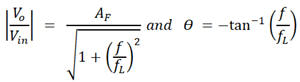
We can use this equation to observe the change in gain magnitude with the change in the frequency of the input signal.

 

Case1: f<<f_L. So let us consider input frequency is very less than the cutoff frequency of the filter then,

So when the input frequency is very less than filter cutoff frequency then gain magnitude is approximately equal to loop gain of the op-amp.

 

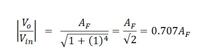
Case2: f = f_L. If the input frequency is equal to the cutoff frequency of the filter then,

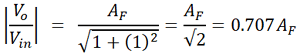
So when the input frequency is equal to filter cutoff frequency then gain magnitude is 0.707 times the loop gain of the op-amp.

 

Case3: f >f_L. If the input frequency is higher than the cutoff frequency of the filter then,

As you can see from the pattern the gain of the filter will be the same as op-amp gain until the input signal frequency is less than the cutoff frequency. But once the input signal frequency reaches cutoff frequency the gain marginally decreases as seen in case two. And as the input signal frequency increases even further the gain gradually decreases until it reaches zero. So the low pass Butterworth filter allows the input signal to appear at the output until the frequency of the input signal is lower than the cutoff frequency.

If we have drawn the frequency response graph for the above circuit we will have,

As seen in the graph, the gain will be linear until the frequency of the input signal crosses the cutoff frequency value and once it happens the gain decreases considerably so does the output voltage value.  

 

Second-Order Butterworth Low Pass Filter

The figure shows the circuit model of the 2nd order Butterworth low pass filter.

 

In the circuit we have:

• Voltage ‘Vin’ as an input voltage signal which is analog in nature.
• Voltage ‘Vo’ is the output voltage of the operational amplifier.
• Resistors ‘RF’ and ‘R1’ are the negative feedback resistors of the operational amplifier.
• There is a double R-C network (marked in a red square) present in the circuit hence the filter is a second-order low pass filter.
• ‘RL’ is the load resistance connected at the op-amp output.

 

Second Order Low Pass Butterworth Filter Derivation 

Second-order filters are important because higher-order filters are designed using them. The gain of the second-order filter is set by R1 and RF, while the cutoff frequency f_H is determined by  R₂, R₃, C₂ & C₃ values. The derivation for the cutoff frequency is given as follows,

fH = 1 / 2ᴫ(R2R3C2C3)1/2

 

The voltage gain equation for this circuit can also be found in a similar way as before and this equation is given below,

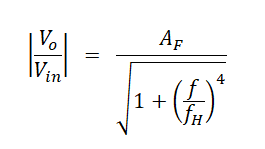
In this equation,

• V₀ / V_in = gain of the filter as a function of frequency
• A_F = (1 + R_F/R₁) passband gain of the filter
• f = frequency of the input signal
• f_H = 1 / 2ᴫ(R₂R₃C₂C₃)^1/2 = cutoff frequency of the filter. We can use this equation to choose appropriate resistor and capacitor values to select the cutoff frequency of the circuit. Also if we choose the same resistor and capacitor in the R-C network then the equation becomes,

We can the voltage gain equation to observe the change in gain magnitude with the corresponding change in the frequency of the input signal.

 

Case1: f<<f_H. So let us consider input frequency is very less than the cutoff frequency of the filter then,

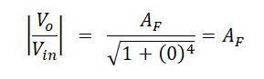
So when the input frequency is very less than filter cutoff frequency then gain magnitude is approximately equal to loop gain of the op-amp.

 

Case2: f = f_H. If the input frequency is equal to the cutoff frequency of the filter then,

So when the input frequency is equal to filter cutoff frequency then gain magnitude is 0.707 times the loop gain of the op-amp.

 

Case3: f >f_H. If the input frequency is really higher than the cutoff frequency of the filter then,

Similar to the first-order filter, the gain of the filter will be the same as op-amp gain up until the input signal frequency is less than the cutoff frequency. But once the input signal frequency reaches cutoff frequency the gain marginally decreases as seen in case two. And as the input signal frequency increases even further the gain gradually decreases until it reaches zero. So the low pass Butterworth filter allows the input signal to appear at the output until the frequency of the input signal is lower than the cutoff frequency.

If we draw the frequency response graph for the above circuit we will have,

Now you might be wondering where is the difference between first-order filter and second-order filter? The answer is in the graph, if you observe carefully you can see after the input signal frequency crosses the cutoff frequency the graph gets a steep decline and this fall is more apparent in the second-order compared to first –order. With this steep inclination, the second-order Butterworth filter will be more inclined towards the ideal filter graph when compared to a single-order Butterworth filter.

This is the same for Third Order Butterworth Low Pass Filter, Forth Order Butterworth Low Pass Filter and so on. The higher the order of the filter the more the gain graph leans to an ideal filter graph. If we draw the gain graph for higher-order Butterworth filters we will have something like this,

In the graph, the green curve represents the ideal filter curve and you can see as the order of the Butterworth filter increases its gain graph leans more towards the ideal curve. So higher the order of Butterworth filter chosen the more ideal the gain curve will be. With that being said you cannot choose a higher-order filter easily as the accuracy of the filter decreases with an increase in the order. Hence it is best to choose the order of a filter while keeping an eye on the required accuracy.

 

 

Second-Order Low Pass Butterworth Filter Derivation -Aliter

After the article was published we received a mail from Keith Vogel, who is a retired electrical engineer. He had noticed a widely publicized error in the description of a 2^nd order low pass filter and offered his explanation to correct it which is as follows. 

So let me get right too it.:

 

And then go to say the -6db cutoff frequency is described by the equation:

fc = 1/()

 

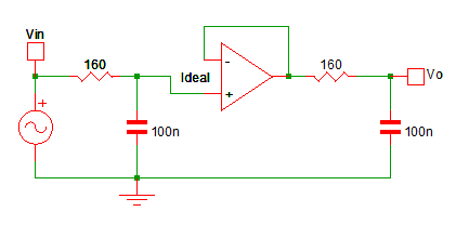
However, this is simply not true! Let’s get you to believe me. Let’s make a circuit where R1=R2=160, and C1=C2=100nF (0.1uF). Given the equation, we should have a -6db frequency of:

fc = 1/()

    = 1/(2*160*100*10-9)

    ~ 9.947kHz

 

Let’s go ahead and simulate the circuit and see where the -6db point is:

 

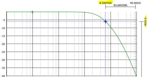
Oh, it simulates to 6.33kHz NOT 9.947kHz; but the simulation is NOT WRONG!

For your information, I have used -6.0206db instead of -6db because 20log(0.5) = -6.0205999132796239042747778944899, -6.0206 is a little closer number than -6, and to get a more accurate simulated frequency to our equations, I wanted to use something a little closer than just -6db. If I really wanted to achieve the frequency outlined by the equation, I would need to buffer between the 1^st and 2^nd stages of the filter. A more accurate circuit to our equation would be:

 

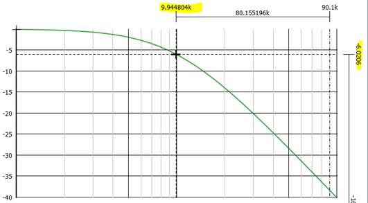
And here we see our -6.0206db point simulates to 9.945kHz, much much closer to our calculated 9.947kHZ. Hopefully, you believe me that there is an error! Now let’s talk about how the error came about, and why this is just bad engineering.

Most descriptions will start with a 1^st order low pass filter, with the impedance as follows.

 

And you get a simple transfer function of:

H(s) = (1/sC)/(R+1/sC) = 1/(sRC+1)

 

Then they say if you just put 2 of these together to make a 2^nd order filter, you get:

H(s) = H1(s) * H2(s).

Where H₁(s) = H₂(s) = 1/(sRC+1)

 

Which when calculated out will result in the fc = 1/(2π√R1C1R2C2) equation. Here is the error, the response of H₁(s) is NOT independent of H₂(s) in the circuit, you can’t say H₁(s) = H₂(s) = 1/(sRC+1).

The impedance of H₂(s) affects the response of H₁(s). And thus why this circuit works, because the opamp isolates H₂(s) from H₁(s)!

 

So now I am going to analyze the following circuit.  Consider our original circuit:

 

For simplicity, I am going to make R1 = R2 and C1 = C2, otherwise, the math gets really involved. But we should be able to derive the actual transfer function and compare it to our simulations for validation when we are done.

  If we say, Z₁ = 1/sC in parallel with (R+1/sC), we can redraw the circuit as:

 

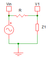
We know that V₁/V_in = Z₁/(R+Z₁); Where Z₁ can be a complex impedance. And if we go back to our original circuit, we can see Z₁ = 1/sC in parallel with (R+1/sC)

 

 

We also can see that Vo/ V₁ = 1/(sRC + 1), which is H₂(s). But H₁(s) Is much more complex, it is Z₁/(R+Z₁)  where Z₁ = 1/sC ||( R+1/sC); and is NOT 1/(sRC+1)! 

So now lets grind through the math for our circuit; for the special case of R1=R2 and C1=C2.

 

 

We have:

V1/Vin = Z1/(R+Z1)

Z1 = 1/sC || (R+1/sC) = (sRC+1)/((sC)2R+2sC)

Vo/ V1 = 1/(sRC + 1)

 

And finally

Vo/Vin = [Z1/(R+Z1)] * [1/(sRC + 1)]

= [(sRC+1)/((sC)2R+2sC)/(R+(sRC+1)/((sC)2R+2sC))] * [1/(sRC + 1)]

= [1/(((sC)2R+2sC)R/(sRC+1) + 1)] * [1/(sRC + 1)]

= [(sRC+1)/((sCR)2+2sRC + sRC + 1)] * [1/(sRC + 1)]

= [(sRC+1)/((sCR)2+3sRC + 1)] * [1/(sRC + 1)]

 

Here we can see that:

H₁(s) = (sRC+1)/((sCR)²+3sRC + 1) …

not 1/(sRC + 1) H₂(s) = 1/(sRC + 1)

 

And..

Vo/Vin = H1(s)* H2(s) = [(sRC+1)/((sCR)2+3sRC + 1)] * [1/(sRC + 1)]

= 1/((sRC)2 + 3sRC + 1)

 

We know that the -6db point is (/2)² = 0.5

And we know when the magnitude of our transfer function is at 0.5, we are at the -6db frequency.

 |Vo/V_in| = 0.5

 

So let’s solve for that:

|Vo/Vin| = |1/((sRC)2 + 3sRC + 1)| = 0.5

 

Let s = jꙍ, we have:

|1/((sRC)2 + 3sRC + 1)| = 0.5

|1/((jꙍRC)2 + 3jꙍRC + 1)| = 0.5

|((jꙍRC)2 + 3jꙍRC + 1)| = 2

|(-(ꙍRC)2 + 3jꙍRC + 1)| = 2

|((1-(ꙍRC)2) + 3jꙍRC| = 2

 

To find the magnitude, take the square root of the square of the real and imaginary terms.

sqrt(((1-(ꙍRC)²)² + (3ꙍRC)²) = 2

squaring both sides:
((1-(ꙍRC)²)² + (3ꙍRC)² = 4

 

Expanding:

1 - 2(ꙍRC)² + (ꙍRC)⁴ + 9(ꙍRC)² = 4

1 + 7(ꙍRC)² + (ꙍRC)⁴ = 4

(ꙍRC)⁴ + 7(ꙍRC)² + 1 = 4

(ꙍRC)⁴ + 7(ꙍRC)² - 3 = 0

 

Let  x = (ꙍRC)²

(x)² + 7x - 3 = 0

 

Using the quadratic equation to solve for x

x = (-7 +/- sqrt(49 – 4*1*(-3)) / 2

= (-7 +/- sqrt(49 +12) / 2

= (-7 +/- ) / 2 = ( - 7) / 2

.. only real answer is the +

 

 

Remember

x = (ꙍRC)2

 

replacing x

(ꙍRC)2 = ( - 7) / 2

ꙍRC = 

ꙍ = ( ) / RC

 

Replacing ꙍ  with 2f_c

 

2f_c =  ( ) / RC

f_c =  ( ) / 2RC  … (-6db) When R1=R2 and C1=C2

 

Ugly, you might not believe me, so read on… For the original circuit I gave you:

 

fc =  ( ) / 2*160*(100*10-9)

fc =  (0.63649417747009060684924081342512) / 2*160*(100*10-9)

fc =  6331.3246620984375557174874117881 ~ 6.331kHz

 

If we go back to our original simulation for this circuit we saw the -6db frequency at ~6.331kHz which lines up exactly to our calculations!

Simulate this for other values, you will see the equation is correct.

 

We can see that when we buffer between the two 1^st order low pass filters we can use the equation

f_c = 1/()

 

And if R1 = R2 and C1 = C2 we can use the equation:

f_c = 1/

 

But if we don’t buffer between the two 1^st order filters our equation (given R1=R2, C1=C2) becomes:

f_c = ( ) / 2RC

f_c ~  0.6365/ 2RC

 

Warning, do not attempt to say:

fc = 0.6365/()

Remember, H₂(s) effects H₁(s); but not the other way around, the filters are not symmetrical, so don’t make this assumption!

 

So if you are going to stay with your current equation, I would recommend a circuit that is more like this: