
- Segmentation and contours
- Hierarchy and retrieval mode
- Approximating contours and finding their convex hull
- Conex Hull
- Matching Contour
- Identifying Shapes (circle, rectangle, triangle, square, star)
- Line detection
- Blob detection
- Filtering the blobs – counting circles and ellipses
1. Segmentation and contours
Image segmentation is a process by which we partition images into different regions. Whereas the contours are the continuous lines or curves that bound or cover the full boundary of an object in an image. And, here we will use image segmentation technique called contours to extract the parts of an image.
Also contours are very much important in
- Object detection
- Shape analysis
And they have very much broad field of application from the real world image analysis to medical image analysis such as in MRI’s
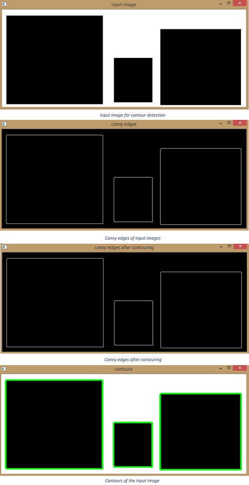
Let’s know how to implement contours in opencv, by extracting contours of squares.
import cv2
import numpy as np
Let’s load a simple image with 3 black squares
image=cv2.imread('squares.jpg')
cv2.imshow('input image',image)
cv2.waitKey(0)
Grayscale
gray=cv2.cvtColor(image,cv2.COLOR_BGR2GRAY)
Find canny edges
edged=cv2.Canny(gray,30,200)
cv2.imshow('canny edges',edged)
cv2.waitKey(0)
Finding contours
#use a copy of your image, e.g. - edged.copy(), since finding contours alter the image
#we have to add _, before the contours as an empty argument due to upgrade of the OpenCV version
_, contours, hierarchy=cv2.findContours(edged,cv2.RETR_EXTERNAL,cv2.CHAIN_APPROX_NONE)
cv2.imshow('canny edges after contouring', edged)
cv2.waitKey(0)
Printing the contour file to know what contours comprises of
print(contours)
print('Numbers of contours found=' + str(len(contours)))
Draw all contours
#use -1 as the 3rd parameter to draw all the contours
cv2.drawContours(image,contours,-1,(0,255,0),3)
cv2.imshow('contours',image)
cv2.waitKey(0)
cv2.destroyAllWindows()
Console Output- [array([[[368, 157]],
[[367, 158]],
[[366, 159]],
...,
[[371, 157]],
[[370, 157]],
[[369, 157]]],
dtype=int32),
array([[[520, 63]],
[[519, 64]],
[[518, 65]],
...,
[[523, 63]],
[[522, 63]],
[[521, 63]]], dtype=int32),array([[[16, 19]],
[[15, 20]],
[[15, 21]],
...,
[[19, 19]],
[[18, 19]],
[[17, 19]]], dtype=int32)]
Numbers of contours found=3. So we have found a total of three contours.
Now, in the above code we had also printed the contour file using [print(contours)], this file tells how these contours looks like, as printed in above console output.
In the above console output we have a matrix which looks like coordinates of x, y points. OpenCV stores contours in a lists of lists. We can simply show the above console output as follows:
CONTOUR 1 CONTOUR 2 CONTOUR 3
[array([[[368, 157]], array([[[520, 63]], array([[[16, 19]],
[[367, 158]], [[519, 64]], [[15, 20]],
[[366, 159]], [[518, 65]], [[15, 21]],
..., ..., ...,
[[371, 157]], [[523, 63]], [[19, 19]],
[[370, 157]], [[522, 63]], [[18, 19]],
[[369, 157]]], dtype=int32), [[521, 63]]], dtype=int32), [[17, 19]]], dtype=int32)]
Now, as we use the length function on contour file, we get the length equal to 3, it means there were three lists of lists in that file, i.e. three contours.
Now, imagine CONTOUR 1 is the first element in that array and that list contains list of all the coordinates and these coordinates are the points along the contours that we just saw, as the green rectangular boxes.
There are different methods to store these coordinates and these are called approximation methods, basically approximation methods are of two types
- cv2.CHAIN_APPROX_NONE
- cv2.CHAIN_APPROX_SIMPLE
cv2.CHAIN_APPROX_NONE stores all the boundary point, but we don’t necessarily need all the boundary points, if the point forms a straight line, we only need the start point and ending point on that line.
cv2.CHAIN_APPROX_SIMPLE instead only provides the start and end points of the bounding contours, the result is much more efficient storage of contour information.
_, contours,hierarchy=cv2.findContours(edged,cv2.RETR_EXTERNAL,cv2.CHAIN_APPROX_NONE)
In the above code cv2.RETR_EXTERNAL is the retrieval mode while the cv2.CHAIN_APPROX_NONE is
the approximation method.
So we have learned about contours and approximation method, now let’s explore hierarchy and retrieval mode.
2. Hierarchy and Retrieval Mode
Retrieval mode defines the hierarchy in contours like sub contours, or external contour or all the contours.
Now there are four retrieval modes sorted on the hierarchy types.
cv2.RETR_LIST – retrieves all the contours.
cv2.RETR_EXTERNAL – retrieves external or outer contours only.
cv2.RETR_CCOMP – retrieves all in a 2-level hierarchy.
cv2.RETR_TREE – retrieves all in a full hierarchy.
Hierarchy is stored in the following format [Next, Previous, First child, parent]
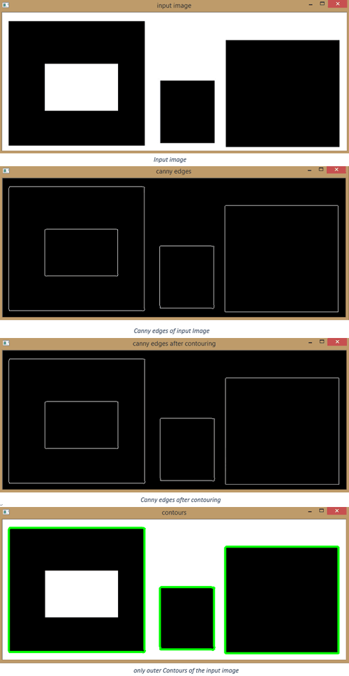
Now let’s illustrate the difference between the first two retrieval modes, cv2.RETR_LIST and cv2.RETR_EXTERNAL.
import cv2
import numpy as np
Lets load a simple image with 3 black squares
image=cv2.imread('square donut.jpg')
cv2.imshow('input image',image)
cv2.waitKey(0)
Grayscale
gray=cv2.cvtColor(image,cv2.COLOR_BGR2GRAY)
Find Canny Edges
edged=cv2.Canny(gray,30,200)
cv2.imshow('canny edges',edged)
cv2.waitKey(0)
Finding Contours
#use a copy of your image, e.g. - edged.copy(), since finding contours alter the image
#we have to add _, before the contours as an empty argument due to upgrade of the open cv version
_, contours,hierarchy=cv2.findContours(edged,cv2.RETR_EXTERNAL,cv2.CHAIN_APPROX_NONE)
cv2.imshow('canny edges after contouring', edged)
cv2.waitKey(0)
Printing the contour file to know what contours comprises of.
print(contours)
print('Numbers of contours found=' + str(len(contours)))
Draw all contours
#use -1 as the 3rd parameter to draw all the contours
cv2.drawContours(image,contours,-1,(0,255,0),3)
cv2.imshow('contours',image)
cv2.waitKey(0)
cv2.destroyAllWindows
Now let’s change the retrieval mode from external to list
import cv2
import numpy as np
Lets load a simple image with 3 black squares
image=cv2.imread('square donut.jpg')
cv2.imshow('input image',image)
cv2.waitKey(0)
Grayscale
gray=cv2.cvtColor(image,cv2.COLOR_BGR2GRAY)
Find canny edges
edged=cv2.Canny(gray,30,200)
cv2.imshow('canny edges',edged)
cv2.waitKey(0)
Finding contours
#use a copy of your image, e.g. - edged.copy(), since finding contours alter the image
#we have to add _, before the contours as an empty argument due to upgrade of the open cv version
_, contours,hierarchy=cv2.findContours(edged,cv2.RETR_LIST,cv2.CHAIN_APPROX_NONE)
cv2.imshow('canny edges after contouring', edged)
cv2.waitKey(0)
Printing the contour file to know what contours comprises of.
print(contours)
print('Numbers of contours found=' + str(len(contours)))
Draw all contours
#use -1 as the 3rd parameter to draw all the contours
cv2.drawContours(image,contours,-1,(0,255,0),3)
cv2.imshow('contours',image)
cv2.waitKey(0)
cv2.destroyAllWindows()
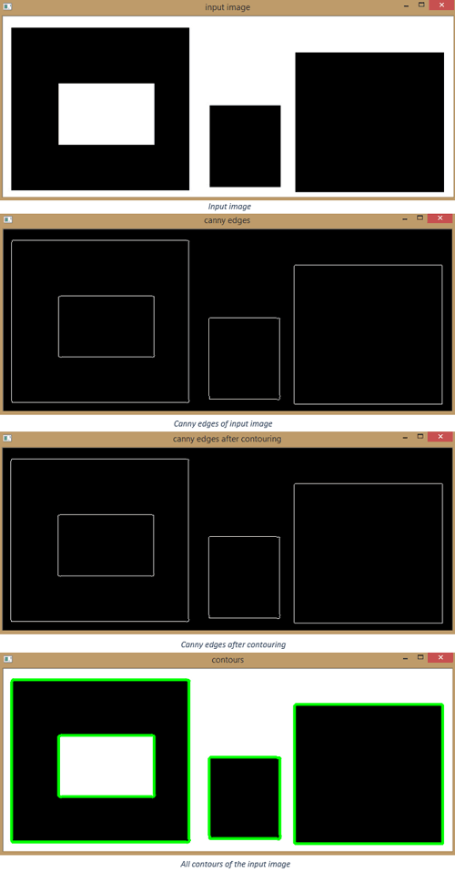
So through the demonstration of above codes we could clearly see the difference between the cv2.RETR_LIST and cv2.RETR_EXTERNNAL, in cv2.RETR_EXTERNNAL only the outer contours are being taken into account while the inner contours are being ignored.
While in cv2.RETR_LIST inner contours are also being taken into account.
3. Approximating Contours and Finding their Convex hull
In approximating contours, a contour shape is approximated over another contour shape, which may be not that much similar to the first contour shape.
For approximation we use approxPolyDP function of openCV which is explained below
cv2.approxPolyDP(contour, approximation accuracy, closed)
Parameters:
- Contour – is the individual contour we wish to approximate.
- Approximation Accuracy- important parameter in determining the accuracy of approximation, small value give precise approximation, large values gives more generic information. A good thumb rule is less than 5% of contour perimeter.
- Closed – a Boolean value that states whether the approximate contour could be open or closed.
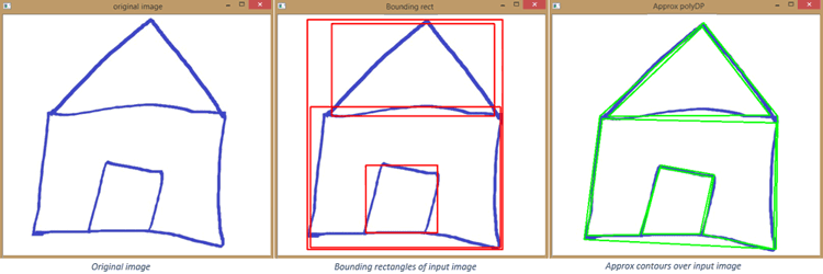
Let’s try to approximate a simple figure of a house
import numpy as np
import cv2
Load the image and keep a copy
image=cv2.imread('house.jpg')
orig_image=image.copy()
cv2.imshow('original image',orig_image)
cv2.waitKey(0)
Grayscale and binarize the image
gray=cv2.cvtColor(image,cv2.COLOR_BGR2GRAY)
ret, thresh=cv2.threshold(gray,127,255,cv2.THRESH_BINARY_INV)
Find Contours
_, contours, hierarchy=cv2.findContours(thresh.copy(),cv2.RETR_LIST,cv2.CHAIN_APPROX_NONE)
Iterate through each contour and compute their bounding rectangle
for c in contours:
    x,y,w,h=cv2.boundingRect(c)
    cv2.rectangle(orig_image,(x,y),(x+w,y+h),(0,0,255),2)
    cv2.imshow('Bounding rect',orig_image)
cv2.waitKey(0)
Iterate through each contour and compute the approx contour
for c in contours:
    #calculate accuracy as a percent of contour perimeter
    accuracy=0.03*cv2.arcLength(c,True)
    approx=cv2.approxPolyDP(c,accuracy,True)
    cv2.drawContours(image,[approx],0,(0,255,0),2)
    cv2.imshow('Approx polyDP', image)
cv2.waitKey(0)
cv2.destroyAllWindows()
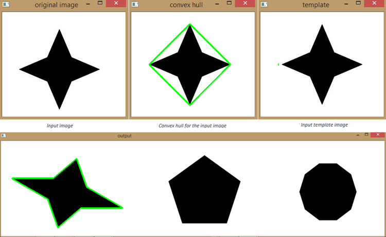
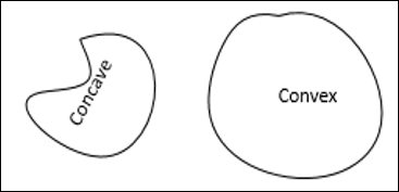
4. Convex Hull
Convex hull is basically the outer edges, represented by drawing lines over a given figure.
It could be the smallest polygon that can fit around the object itself.
import cv2
import numpy as np
image=cv2.imread('star.jpg')
gray=cv2.cvtColor(image,cv2.COLOR_BGR2GRAY)
cv2.imshow('original image',image)
cv2.waitKey(0)
Threshold the image
ret, thresh=cv2.threshold(gray,176,255,0)
Find contours
_, contours, hierarchy=cv2.findContours(thresh.copy(),cv2.RETR_LIST,cv2.CHAIN_APPROX_NONE)
Sort the contours by area and then remove the largest frame contour
n=len(contours)-1
contours=sorted(contours,key=cv2.contourArea,reverse=False)[:n]
Iterate through the contours and draw convex hull
for c in contours:
    hull=cv2.convexHull(c)
    cv2.drawContours(image,[hull],0,(0,255,0),2)
    cv2.imshow('convex hull',image)
    cv2.waitKey(0)
    cv2.destroyAllWindows()
5. Matching Contour by shapes
cv2.matchShapes(contour template, contour method, method parameter)
Output – match value(lower value means a closer match)
contour template – This is our reference contour that we are trying to find in a new image.
contour – The individual contour we are checking against.
Method – Type of contour matching (1,2,3).
method parameter – leave alone as 0.0 (not utilized in python opencv)
import cv2
import numpy as np
Load the shape template or reference image
template= cv2.imread('star.jpg',0)
cv2.imshow('template',template)
cv2.waitKey(0)
Load the target image with the shapes we are trying to match
target=cv2.imread('shapestomatch.jpg')
gray=cv2.cvtColor(target,cv2.COLOR_BGR2GRAY)
Threshold both the images first before using cv2.findContours
ret,thresh1=cv2.threshold(template,127,255,0)
ret,thresh2=cv2.threshold(gray,127,255,0)
Find contours in template
_,contours,hierarhy=cv2.findContours(thresh1,cv2.RETR_CCOMP,cv2.CHAIN_APPROX_SIMPLE)
#we need to sort the contours by area so we can remove the largest contour which is
Image outline
sorted_contours=sorted(contours, key=cv2.contourArea, reverse=True)
#we extract the second largest contour which will be our template contour
tempelate_contour=contours[1]
#extract the contours from the second target image
_,contours,hierarchy=cv2.findContours(thresh2,cv2.RETR_CCOMP,cv2.CHAIN_APPROX_SIMPLE)

for c in contours:
    #iterate through each contour in the target image and use cv2.matchShape to compare the contour shape
    match=cv2.matchShapes(tempelate_contour,c,1,0.0)
    print("match")
    #if match value is less than 0.15
    if match<0.16:
        closest_contour=c
    else:
        closest_contour=[]

cv2.drawContours(target,[closest_contour],-1,(0,255,0),3)
cv2.imshow('output',target)
cv2.waitKey(0)
cv2.destroyAllWindows()
Console Output –
0.16818605122199104
0.19946910256158912
0.18949760627309664
0.11101058276281539
There are three different method with different mathematics function, we can experiment with each method by just replacing cv2.matchShapes(tempelate_contour,c,1,0.0) method values which varies from 1,2 and 3, for each value you will get different match values in console output.

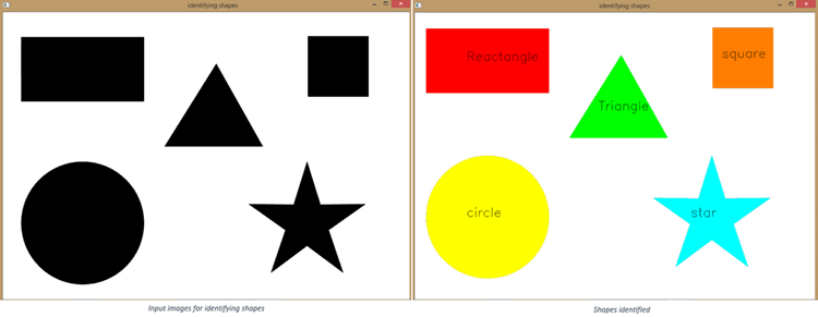
6. Identifying Shapes (circle, rectangle, triangle, square, star)
OpenCV can also be used for detecting different types of shapes automatically from the image. By using below code we will be able to detect circle, rectangle, triangle, square and stars from the image.
import cv2
import numpy as np
Load and then gray scale images
image=cv2.imread('shapes.jpg')
gray=cv2.cvtColor(image,cv2.COLOR_BGR2GRAY)
cv2.imshow('identifying shapes',image)
cv2.waitKey(0)

ret, thresh=cv2.threshold(gray,127,255,1)
Extract contours
_,contours,hierarchy=cv2.findContours(thresh.copy(),cv2.RETR_LIST,cv2.CHAIN_APPROX_NONE)
For cnt in contours:
 Get approximate polygons
    approx = cv2.approxPolyDP(cnt,0.01*cv2.arcLength(cnt,True),True)
    if len(approx)==3:
        shape_name="Triangle"
        cv2.drawContours(image,[cnt],0,(0,255,0),-1)
find contour center to place text at the center
        M=cv2.moments(cnt)
        cx=int(M['m10']/M['m00'])
        cy=int(M['m01']/M['m00'])
        cv2.putText(image,shape_name,(cx-50,cy),cv2.FONT_HERSHEY_SIMPLEX,1,(0,0,0),1)
     elif len(approx)==4:
        x,y,w,h=cv2.boundingRect(cnt)
        M=cv2.moments(cnt)
        cx=int(M['m10']/M['m00'])
        cy=int(M['m01']/M['m00'])
Check to see if that four sided polygon is square or rectangle
        #cv2.boundingRect return the left width and height in pixels, starting from the top
        #left corner, for square it would be roughly same
        if abs(w-h) <= 3:
            shape_name="square"
            #find contour center to place text at center
            cv2.drawContours(image,[cnt],0,(0,125,255),-1)
            cv2.putText(image,shape_name,(cx-50,cy),cv2.FONT_HERSHEY_SIMPLEX,1,(0,0,0),1)
        else:
            shape_name="Reactangle"
            #find contour center to place text at center
            cv2.drawContours(image,[cnt],0,(0,0,255),-1)
            M=cv2.moments(cnt)
            cx=int(M['m10']/M['m00'])
            cy=int(M['m01']/M['m00'])
            cv2.putText(image,shape_name,(cx-50,cy),cv2.FONT_HERSHEY_SIMPLEX,1,(0,0,0),1)
    elif len(approx)==10:
        shape_name='star'
        cv2.drawContours(image,[cnt],0,(255,255,0),-1)
        M=cv2.moments(cnt)
        cx=int(M['m10']/M['m00'])
        cy=int(M['m01']/M['m00'])
        cv2.putText(image,shape_name,(cx-50,cy),cv2.FONT_HERSHEY_SIMPLEX,1,(0,0,0),1)
    elif len(approx)>=15:
        shape_name='circle'
        cv2.drawContours(image,[cnt],0,(0,255,255),-1)
        M=cv2.moments(cnt)
        cx=int(M['m10']/M['m00'])
        cy=int(M['m01']/M['m00'])
        cv2.putText(image,shape_name,(cx-50,cy),cv2.FONT_HERSHEY_SIMPLEX,1,(0,0,0),1)
    cv2.imshow('identifying shapes', image)
    cv2.waitKey(0)
cv2.destroyAllWindows()
7. Line Detection
Line detection is very much important concept in OpenCV, and has a promising use in the real world. Autonomous cars use line detection algorithms for the detection of lanes and roads.
In line detection we will deal with two algorithms,
- Hough Line Algorithm
- Probalistic Hough Line Algorithm.
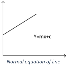
You may have remembered the representation of line from high school mathematics with the equation, y=mx+c.
However, in OpenCV line is represented by another way
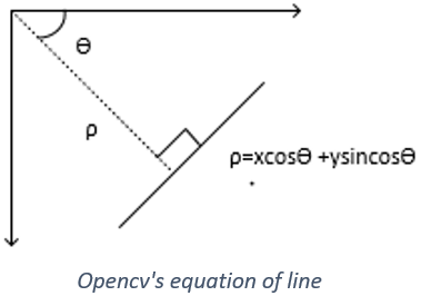
The equation above ρ=xcosӨ +ysincosӨ is the OpenCV representation of the line, wherein ρ is the perpendicular distance of line from origin and Ө is the angle formed by the normal of this line to the origin (measured in radians, wherein 1pi radians/180 = 1 degree).
The OpenCV function for the detection of line is given as
cv2.HoughLines(binarized image, ρ accuracy, Ө accuracy, threshold), wherein threshold is minimum vote for it to be considered a line.
Now let’s detect lines for a box image with the help of Hough line function of opencv.
import cv2
import numpy as np
image=cv2.imread('box.jpg')
Grayscale and canny edges extracted
gray=cv2.cvtColor(image,cv2.COLOR_BGR2GRAY)
edges=cv2.Canny(gray,100,170,apertureSize=3)
Run Hough lines using rho accuracy of 1 pixel
#theta accuracy of (np.pi / 180) which is 1 degree
#line threshold is set to 240(number of points on line)
lines=cv2.HoughLines(edges, 1, np.pi/180, 240)
#we iterate through each line and convert into the format
#required by cv2.lines(i.e. requiring end points)
for i in range(0,len(lines)):
for rho, theta in lines[i]:
a=np.cos(theta)
b=np.sin(theta)
x0=a*rho
y0=b*rho
x1=int(x0+1000*(-b))
y1=int(y0+1000*(a))
x2=int(x0-1000*(-b))
y2=int(y0-1000*(a))
cv2.line(image,(x1,y1),(x2,y2),(0,255,0),2)
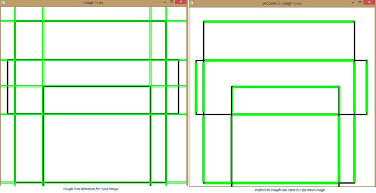
cv2.imshow('hough lines',image)
cv2.waitKey(0)
cv2.destroyAllWindows()
Now let’s repeat above line detection with other algorithm of probabilistic Hough line.
The idea behind probabilistic Hough line is to take a random subset of points sufficient enough for line detection.
The OpenCV function for probabilistic Hough line is represented as cv2.HoughLinesP(binarized image, ρ accuracy, Ө accuracy, threshold, minimum line length, max line gap)
Now let’s detect box lines with the help of probabilistic Hough lines.
import cv2
import numpy as np
Grayscale and canny edges Extracted
image=cv2.imread('box.jpg')
gray=cv2.cvtColor(image,cv2.COLOR_BGR2GRAY)

edges=cv2.Canny(gray,50,150,apertureSize=3)
#again we use the same rho and theta accuracies
#however, we specify a minimum vote(pts along line) of 100
#and min line length of 5 pixels and max gap between the lines of 10 pixels

lines=cv2.HoughLinesP(edges,1,np.pi/180,100,100,10)
for i in range(0,len(lines)):
    for x1,y1,x2,y2 in lines[i]:
        cv2.line(image,(x1,y1),(x2,y2),(0,255,0),3)

cv2.imshow('probalistic hough lines',image)
cv2.waitKey(0)
cv2.destroyAllWindows
8. Blob detection
Blobs can be described as a group of connected pixels that all share a common property. The method to use OpenCV blob detector is described through this flow chart.
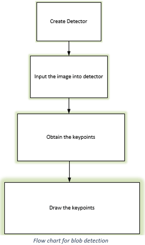
For drawing the key points we use cv2.drawKeypoints which takes the following arguments.
cv2.drawKeypoints(input image,keypoints,blank_output_array,color,flags)
where in the flags could be
cv2.DRAW_MATCHES_FLAGS_DEFAULT
cv2.DRAW_MATCHES_FLAGS_DRAW_RICH_KEYPOINTS
cv2.DRAW_MATCHES_FLAGS_DRAW_OVER_OUTIMG
cv2.DRAW_MATCHES_FLAGS_NOT_DRAW_SINGLE_POINTS
and blank here is pretty much nothing but one by one matrix of zeros
Now let’s perform the blob detection on an image of sunflowers, where the blobs would be the central parts of the flower as they are common among all the flowers.
import cv2
import numpy as np
image=cv2.imread('Sunflowers.jpg',cv2.IMREAD_GRAYSCALE)
Set up detector with default parameters
detector=cv2.SimpleBlobDetector_create()
Detect blobs
keypoints= detector.detect(image)
Draw detected blobs as red circles
#cv2.DRAW_MATCHES_FLAGS_DRAW_RICH_KEYPOINTS ensure the
#size of circle corresponds to the size of blob
blank=np.zeros((1,1))
blobs=cv2.drawKeypoints(image,keypoints,blank,(0,255,255),cv2.DRAW_MATCHES_FLAGS_DEFAULT)
Show keypoints
cv2.imshow('blobs',blobs)
cv2.waitKey(0)
cv2.destroyAllWindows()
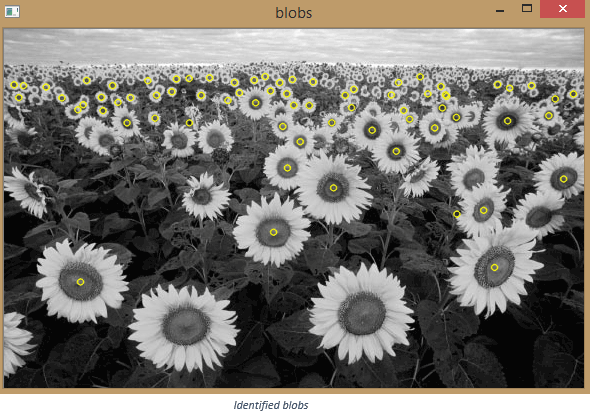
Even though the code works fine but some of the blobs are missed due to uneven sizes of the flowers as the flowers in the front are big as compared to the flowers at the end.
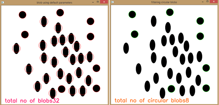
9. Filtering the Blobs – Counting Circles and Ellipses
We can use parameters for filtering the blobs according to their shape, size and color. For using parameters with blob detector we use the OpenCV’s function
cv2.SimpleBlobDetector_Params()
We will see filtering the blobs by mainly these four parameters listed below:
Area
params.filterByArea=True/False
params.minArea=pixels
params.maxArea=pixels
Circularity
params.filterByCircularity=True/False
params.minCircularity=  1 being perfect, 0 being opposite
Convexity - Area of blob/area of convex hull
params.filterByConvexity= True/False
params.minConvexity=Area
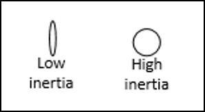
Inertia
params.filterByInertia=True/False
params.minInertiaRatio=0.01
Now let’s try to filter blobs by above mentioned parameters
import cv2
import numpy as np
image=cv2.imread('blobs.jpg')
cv2.imshow('original image', image)
cv2.waitKey(0)
Initialize the detector using default parameters
detector=cv2.SimpleBlobDetector_create()
Detect blobs
keypoints=detector.detect(image)
Draw blobs on our image as red circles
blank=np.zeros((1,1))
blobs=cv2.drawKeypoints(image,keypoints,blank,(0,0,255),cv2.DRAW_MATCHES_FLAGS_DRAW_RICH_KEYPOINTS)

number_of_blobs=len(keypoints)
text="total no of blobs"+str(len(keypoints))
cv2.putText(blobs,text,(20,550),cv2.FONT_HERSHEY_SIMPLEX,1,(100,0,255),2)
Display image with blob keypoints
cv2.imshow('blob using default parameters',blobs)
cv2.waitKey(0)
Set our filtering parameters
#initialize parameter setting using cv2.SimpleBlobDetector
params=cv2.SimpleBlobDetector_Params()
Set area filtering parameters
params.filterByArea=True
params.minArea=100
Set circularity filtering parameters
params.filterByCircularity=True
params.minCircularity=0.9
Set convexity filtering parameter
params.filterByConvexity=False
params.minConvexity=0.2
Set inertia filtering parameter
params.filterByInertia=True
params.minInertiaRatio=0.01
Create detector with parameter
detector=cv2.SimpleBlobDetector_create(params)
Detect blobs
keypoints=detector.detect(image)
Draw blobs on the images as red circles
blank=np.zeros((1,1))
blobs=cv2.drawKeypoints(image,keypoints,blank,(0,255,0),cv2.DRAW_MATCHES_FLAGS_DRAW_RICH_KEYPOINTS)
number_of_blobs=len(keypoints)
text="total no of circular blobs"+str(len(keypoints))
cv2.putText(blobs,text,(20,550),cv2.FONT_HERSHEY_SIMPLEX,1,(0,100,255),2)
Show blobs
cv2.imshow('filtering circular blobs',blobs)
cv2.waitKey(0)
cv2.destroyAllWindows()
So this is how Image segmentation can be done in Python-OpenCV. To get good understating of computer vision and OpenCV, go through previous articles (Getting started with Python OpenCV and Image Manipulations in Python OpenCV and you will be able to make something cool with Computer Vision.
I've gotten as far as number 5, but there are a couple of issues with it:
1. sorted_contours = sorted(contours, key=cv2.contourArea, reverse=True)
but then you never use the sorted array, and instead mistakenly use just "contours", in the next line, which should be: template_contour = sorted_contours[1]
2. In your for...in loop, you set closest_contour to "c" if the match spec is good, but then to an empty list if not. So if the last checked contour is not a matching contour, you will wipe out any good contour match you might have. Additionally if no match is found, parameter 2 of drawContours becomes invalid, causing a fatal exception.
So far though, I have to say this has been a really great article on segmentation.

Really informative article... thanks..☺️