RF Engineering is one of the most interesting and challenging parts of Electrical Engineering due to its high computational complexity of nightmarish tasks like impedance matching of interconnected blocks, associated with the practical implementation of RF solutions. In today’s age with different software tools, things are a bit easier but if you go back to the periods before computers became this powerful, you will understand how difficult things were. For today’s tutorial, we will be looking at one of the tools that were developed back then and are still currently being used by engineer for RF designs, behold The Smith Chart. We will look into the types of smith chart, its construction and how to make sense of the data it holds.
What is a Smith Chart?
The Smith Chart, named after its Inventor Phillip Smith, developed in the 1940s, is essentially a polar plot of the complex reflection coefficient for arbitrary impedance.
It was originally developed to be used for solving complex maths problem around transmission lines and matching circuits which has now been replaced by computer software. However, the Smith charts method of displaying data have managed to retain its preference over the years and it remains the method of choice for displaying how RF parameters behave at one or more frequencies with the alternative being tabulating the information.
Smith chart can be used to display several parameters including; impedances, admittances, reflection coefficients, scattering parameters, noise figure circles, constant gain contours and regions for unconditional stability, and mechanical vibrations analysis, all at the same time. As a result of this, most RF Analysis Software and simple impedance measuring instruments include smith charts in the display options which makes it an important topic for RF Engineers.
Types of Smith Charts
Smith chart is plotted on the complex reflection coefficient plane in two dimensions and is scaled in normalised impedance (the most common), normalised admittance or both, using different colours to distinguish between them and serving as a means to categorize them into different types. Based on this scaling, smith charts can be categorized into three different types;
- The Impedance Smith Chart (Z Charts)
- The Admittance Smith Chart (YCharts)
- The Immittance Smith Chart. (YZ Charts)
While the impedance smith charts are the most popular and the others rarely get a mention, they all have their “superpowers” and can be extremely useful when used interchangeably. To go over them one after the other;
1. Impedance Smith Chart
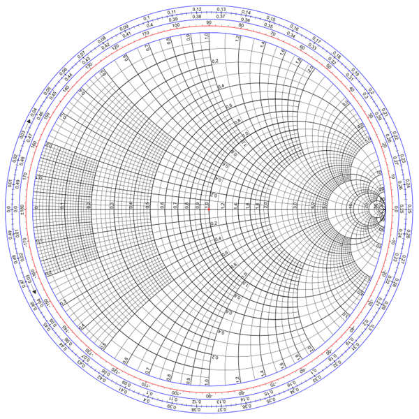
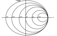
The Impedance smith charts are usually referred to as the normal smith charts since they relate with impedance and works really well with loads made up of series components, which are usually the main elements in impedance matching and other related RF engineering tasks. They are the most popular, with all references to smith charts usually pointing to them and others being regarded as derivatives. The image below shows an impedance smith chart.
The focus of today’s article will be on them so more details will be provided as the article proceeds.
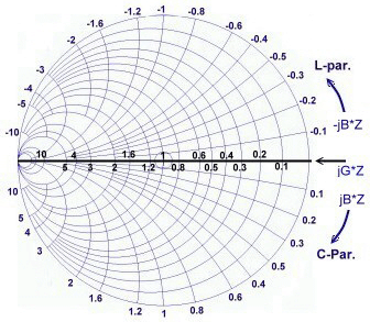
2. Admittance Smith Chart
The Impedance chart is great when dealing with load in series as all you need to do is simply add the impedance up, but the math becomes really tricky when working with parallel components( parallel inductors, capacitors or shunt transmission lines). To allow the same simplicity, the admittance chart was developed. From basic electricity classes, you will remember that admittance is the inverse of impedance as such, an admittance chart makes sense for the complex parallel situation as all you will need to do is to examine the admittance of the antenna rather than the impedance and just add them up. An equation to establish the relationship between admittance and impedance is shown below.
YL = 1 / ZL = C + iS …….(1)
Where YL is the admittance of the load, ZL is the impedance, C is the real part of the admittance known as Conductance, and S is the imaginary part known as Susceptance. True to their relationship described by the relationship above, the admittance smith chart possesses an inverse orientation to the Impedance smith chart.
The image below shows the admittance Smith Chart.
3. The Immittance Smith Chart
The complexity of the smith chart increases down the list. While the “common” impedance Smith Chart is super useful when working with series components and the admittance Smith Chart is great for parallel components, a unique difficulty is introduced when both series and parallel components are involved in the setup. To solve this, the immittance smith chart is used. Its a literally effective solution to the problem as it is formed by superimposing both the Impedance and Admittance smith charts on one another. The picture below shows a typical Immittance Smith Chart.
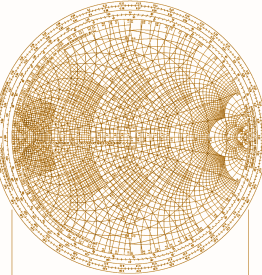
It is as useful as combining the ability of both the admittance and impedance smith charts can be. In Impedance matching activities, it helps identify how a parallel or series component affects the impedance with less effort.
Smith Chart Basics
As mentioned in the introduction, the Smith Chart displays the complex reflection coefficient, in polar form, for a particular load impedance. Going back to basic electricity classes, you will remember that impedance is a sum of resistance and reactance and as such, is more often than not, a complex number, as a result of this, the reflection coefficient is also a complex number, since it is completely determined by the impedance ZL and the "reference" impedance Z0.
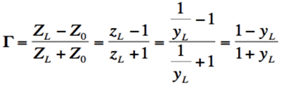
Based on this, the reflection coefficient can be obtained by the equation;
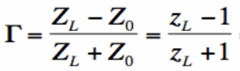
Where Zo is the impedance of the transmitter (or whatever is delivering power to the antenna) while ZL is the impedance of the load.
Hence, the Smith Chart is essentially a graphical method of displaying the impedance of an antenna as a function of frequency, either as a single point or a range of points.
Components of a Smith Chart
A typical smith chart is scary to look at with lines going here and there but it becomes easier to appreciate it once you understand what each line represents.
Impedance Smith Chart
Impedance Smith Chart contains two major elements which are the two circles/arcs which define the shape and data represented by the Smith Chart. These circles are known as;
- The Constant R Circles
- The Constant X Circles
1. The Constant R Circles
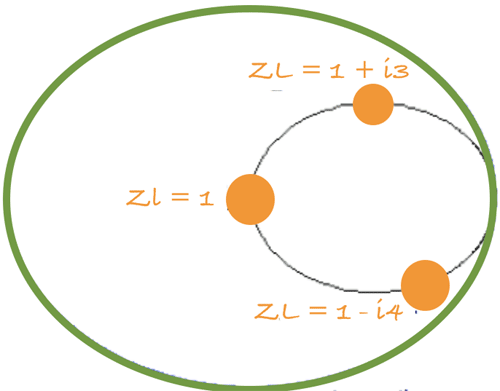
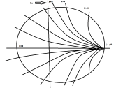
The first set of lines referred to as Constant Resistance lines form circles, all tangent to each other at the right hand of horizontal diameter. The constant R Circles are essentially what you get when the Resistance part of the Impedance is held constant, while the value of X varies. As such, all the points on a particular Constant R circle represent the same resistance value(Fixed Resistance) . The value of the resistance represented by each Constant R Circle is marked on the horizontal line, at the point where the circle intersects with it. It is usually given by the diameter of the circle.
For example, consider a normalized impedance, ZL = R + iX, If R was equal to one and X was equal to any real number such that, ZL = 1 +i0, ZL = 1 +i3, and ZL = 1 +i4, a plot of the impedance on the smith chart will look like the image below.
Plotting multiple constant R Circles gives an image similar to the one below.
This should give you an idea of how the giant circles in the smith chart is generated. The Innermost and Outermost Constant R Circles, represent the boundaries of the smith chart. The Innermost Circle(black) is referred to as the infinite resistance, while the outermost circle is referred to as the zero resistance.
2. The Constant X Circles
The Constant X Circles are more of arcs than circles and are all tangent to each other on the right-hand extreme of horizontal diameter. They are generated when the impedance has a fixed reactance but a varying value of resistance.
The lines in the upper half represent positive reactances while those in the lower half represent negative reactances.
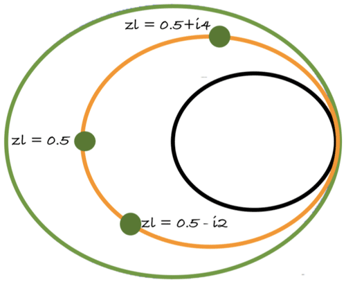
For example, let us consider a curve defined by ZL = R + iY, if Y = 1 and held constant while R representing a real number, is varied from 0 to infinity is plotted(blue line) on the Constant R Circles generated above, a plot similar to the one in the image below is obtained.
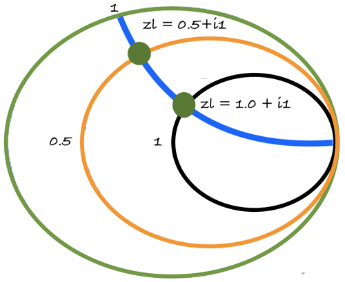
Plotting multiple values of ZL for both the curves, we get a smith chart similar to the one in the image below.
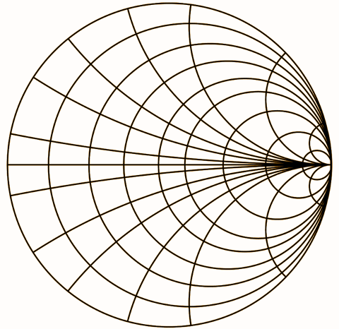
Thus, a complete Smith Chart is obtained by when these two circles described above are superimposed on one another.
Admittance Smith Chart
For Admittance Smith Charts, the inverse is the case. The admittance relative to the impedance is given by the equation 1 above as such, the admittance is made up of Conductance and succeptance which means in the case of the admittance smith chart, rather than having the Constant Resistance Circle, we have the Constant Conductance Circle and rather than having the Constant Reactance circle, we have the Constant Succeptance circle.
Note that the admittance Smith Chart will still plot the reflection coefficient but the direction and location of the graph will be opposite to that of the Impedance smith chart as mathematically established in the equation below
 …… (3)
To better explain this, let’s consider the normalized admittance Yl = G + i*S G = 4(Constant) and S is any real number. Creating the constant conductance plot of the smith using equation 3 above to obtain the reflection coefficient and plotting for different values of S, we get the smith chart shown below.
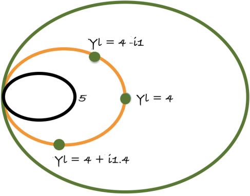
The same thing holds for the Constant Succeptance Curve. If the variable S = 4(Constant) and G is a real number, a plot of the Constant susceptance curve(red) superimposed on the Constant Conductance curve will look like the image below.
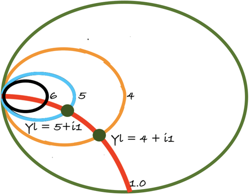
Thus, the Admittance Smith Chart will be an inverse of the Impedance smith chart.
The Smith chart also has circumferential scaling in wavelengths and degrees. The wavelength scale is used in distributed component problems and represents the distance measured along the transmission line connected between the generator or source and the load to the point under consideration. The degrees scale represents the angle of the voltage reflection coefficient at that point.
Applications of Smith Charts
Smith charts find applications in all areas of RF Engineering. Some of the most popular application includes;
- Impedance calculations on any transmission line, on any load.
- Admittance calculations on any transmission line, on any load.
- Calculation of the length of a short circuited piece of transmission line to provide a required capacitive or inductive reactance.
- Impedance matching.
- Determining VSWR among others.
How to use Smith Charts for Impedance matching
Using a Smith chart and interpreting the results derived from it requires a good understanding of AC circuit and transmission line theories, both of which are natural pre-requisite for RF engineering. As an example of how smith charts, are used, we will look at one of it’s most popular use cases which is impedance matching for antennas and transmission lines.
In solving problems around matching, the smith chart is used to determine the value of the component (capacitor or inductor) to use to ensure the line is perfectly matched, that is, ensuring the reflection coefficient is zero.
For example, Let’s assume an impedance of Z = 0.5 - 0.6j. The first task to do will be to find the 0.5 constant resistance circle on the smith chart. Since the impedance has a negative complex value, implieing a capacitive impedance, you will need to move counter-clockwise along the 0.5 resistance circle to find the point where it hits the -0.6 constant reactance arc (if it were a positive complex value, it would represent an inductor and you would move clockwise).This then gives an idea of the value of the components to use to match the load to the line.
Normalised scaling allows the Smith chart to be used for problems involving any characteristic or system impedance, which is represented by the center point of the chart. For Impedance smith charts, the most commonly used normalization impedance is 50 ohms and it opens the graph up making tracing the impedance easier. Once an answer is obtained through the graphical constructions described above, it is straightforward to convert between normalised impedance (or normalised admittance) and the corresponding unnormalized value by multiplying by the characteristic impedance (admittance). Reflection coefficients can be read directly from the chart as they are unit-less parameters.
Also, the value of impedances and admittances change with frequency and the complexity of problems involving them increases with frequency. Smith charts can however be used to solve these problems, one frequency at a time or over multiple frequencies.
When solving the problem manually with one frequency at a time, the result is usually represented by a point on the chart. While these are sometimes “enough” for narrow bandwidth applications, it is usually a difficult approach for application with Wide Bandwidth involving several frequencies. As such the smith Chart is applied over a wide range of frequencies and the result is represented as a Locus (connecting several points) rather than a single point, provided the frequencies are close.
These locus of points covering a range of frequencies on the smith chart can be used to visually represent:
- How capacitive or inductive a Load is across the examined frequency range
- How difficult matching is likely to be at the various frequencies
- How well-matched a particular component is.
The accuracy of the Smith chart is reduced for problems involving a large locus of impedances or admittances, although the scaling can be magnified for individual areas to accommodate these.
The Smith chart may also be used for lumped element matching and analysis problems.